Download

1 / 75
750 likes | 855 Views
AGE 411: Hydrology. Introduction Hydrology is an earth science. It encompasses the occurrence, distribution, movement and properties of the waters of the earth and their environmental relationships. Introduction Contnd: Hydrologic Cycle.

E N D
AGE 411: Hydrology Introduction Hydrology is an earth science. It encompasses the occurrence, distribution, movement and properties of the waters of the earth and their environmental relationships.
Introduction Contnd:Hydrologic Cycle. • Is a continuous process by which water is transported from the oceans to the atmosphere, to the land and back to the sea. • Many such cycles exist - the evaporation of inland water and its subsequent precipitation over land before returning to the ocean is one example.
Hydrologic Cycle Contnd. - the driving force for the global water transport system is provided by the sun, which furnishes the energy required for evaporation. The complete water cycle is global in nature. World water problems require studies on regional, national, international, continental and global scales. PROBLEM? – Practical significance of the fact that the total supply of fresh water available to the earth is limited and very small compared with the small water content of the ocean has received little attention. Thus water flowing in one country can not be available at the same time for use in other regions of the world.
Hydrologic Cycle Contnd. • Water resources are a global problem with local roots. Therefore, developing techniques to control weather must receive careful attention, since climatologically changes in one area can profoundly affect the hydrology and therefore the water resources of other regions.
Introduction Contd. • The Hydrologic Budget: Because the total quantity of water available to the earth is finite and indestructible, the global hydrologic system may be looked upon as closed. However, open hydrologic subsystems are abundant and these are usually the types analyzed by the engineering hydrologist.
Introduction Contd. • Hydrologic Budget Contd. For a system, a water budget can be developed to account for the hydrologic components. Assumptions: a). Perfect plane b). Completely impervious plane c). Confined on all 4 sides with an outlet
Introduction Contd. • Hydrologic Budget Contd. As a perfect plane, it means there is no depressions in which water can be stored. If rain input is applied, and output designed as outflow, surface runoff will be developed at A. Then the hydrologic budget for an open system can be represented by: I – Q = ds/dt Where; I = inflow/unit time, Q = outflow/unit time ds/dt = change in storage in the system/unit time.
Introduction Contd. • Hydrologic Budget Contd. Until a minimal depth is accumulated on the Surface, outflow can not occur, but as storm intensifies, the depth retained on the surface increases. At the cessation of input, water held on the surface becomes the outflow from the system. For this example, all input becomes output, neglecting the small quantity bonded in the surface
Introduction Contd. • Hydrologic Budget Contd. This is always misleading as will be seen later that the terms in the equation can not always be adequately or easily quantified. A more generalized version explains all the components of the hydrologic cycle. Hydrologic budget for a region can be written as: P – R – G – E – T = S ( Basic equation) where; P = precipitation, R = Runoff, G = Groundwater flow, E = Evaporation, T = Transpiration, S = storage.
Introduction Contd. • Application: Question: In a given year, 12,560km2 Watershed received 50.8cms of precipitation The annual rate of flow measured in the river draining the area was found to be 20.57cms. Make a rough estimate of the combined amounts of water evaporated and transpired from the region during the year.
Introduction Contd. • Solution: P – R – G – E – T = S since evap. and transp. can be combined, ET = P – R – G - S Assumptions: 1). Drainage area is quite large, G component may be assumed Zero. 2). That S = 0 Then ET = P – R = 50.8 – 20.57 = 30.23cm/year
Introduction Contd. • Question (2): The storage in a river reach at a given time is 19,734.m3. At the same time, the inflow is 14.15m3/s and the outflow is 19.81m3/s. One hr. later, the inflow rate is 19.81m3/s and outflow is 20.942m3/s. Determine the change in storage in the reach that occurred during the hour. Is the storage at the end of the hour > or < the original value?
Introduction Contd. • Solution to Question(2): I – O = S/T ( continuity for the time interval) (I1 +I2)/2 – (O1 + O2)/2 = (S2 – S1)/t 14.15+19.81–19.81 + 20.94 = s2 -19,734m3 3600sec
Precipitation • Occurs primarily in the form of: 1). Rain 2) Snow 3). Drizzle and 4). Hail 1). Rainfall • An extremely variable quantity. • Problem? – How to deal with variability • Rainfall is random and stochastic • Rainfall is variable both spatially and temporarily i.e. varies in space and time.
Precipitation Contd. • Rainfall Contd. • Formation: There are three types of formation: a). Convective occurrence – this is primarily due to a lifting mechanism by which warm light air rises and mixes with colder denser air. b). Cyclonic formation: This occurs when lifting mechanism occurs because of air rising and meeting with low pressure area eg: cyclone. c). Orographic formation: This is due to lifting of air masses over barriers such as mountains.
Precipitation Contd. • Rainfall Contd. Measurement – There are basically two ways of measurement: • Non – recording gauges. What is obtained is the depth of rain that occurs on periodic basis eg:- standard rain gauge with no time history of the event. 2). Recording gauges This gives rainfall rate because it gives a continuous record of the event with time. i). Tipping bucket; ii). Weighing bucket, iii).Radar type Data useful from recording gauges. -good for rainfall runoff modeling - gives better information due to rainfall variability
Precipitation Contd. • Rainfall Contd. - Error Analysis: Main physical parameters causing error are: 1). Evaporation, 2). Inclination, 3). Splashing 4). Adhesion, 5). Wind • Given any basin, there is problem of estimating point rainfall and basin precipitation. There is also problem of estimating Basin precipitation based on the data available in the Basin. • Point rainfall is needed for: a). Estimating missing data – It may mean record not collected due to measurement problems. b). Constructing depth-duration frequency curves called DDF and Intensity-duration frequency curves called IDF.
Precipitation Contd. • Rainfall contd. • Estimating Point Rainfall: In estimating point rainfall, the method of weighted averages is often used. This gives depth of rainfall that is smaller than the greatest amount and larger than the smallest amount of the area. i.e. lies between Pmax and Pmin of the area.
Precipitation Contd. • Estimating Point Rainfall Contd. Method: Consider that rainfall is to be calculated for point A. Establish a set of axes running through A and determine the absolute coordinates of the nearest surrounding points BCDEF. The estimated precipitation at A is determined as a weighted average of the other five points. The weights are reciprocals of the sums of the squares of X and Y, that is D2 = X2 + y2 and W = 1/D2 The estimated rainfall at the point of interest is given by: ( P x W )/ W
Precipitation Contd. • Example of Point Rainfall Determination: Point Rainfall X Y X2 + Y2 D2 W P x W ( mm ) (m) (m) A - - - - - - - B 160 40 20 C 180 10 16 D 150 30 20 E 200 30 30 F 170 20 20 Sums W P x W Estimated Precipitation of A = PxW / W
Precipitation Contd. • Method of Estimating Point Rainfall: 1). Draw X and Y axis through the interested point 2). Mark up the distances along the X and Y axis. 3). Put them down (distances along the ordinates) 4). Calculate D2 = X2 + Y2 5). Calculate W = 1/D2 6). Have the sum of (PxW) i.e. (PxW) 7). Rainfall at the point = (PxW)/W
Aerial Precipitation • For most hydrologic analyses, it is important to know the aerial distribution of precipitation. Usually, the average depth for representative portions of the watershed are determined and used for this purpose. • The most direct approach is to use the arithmetic average of gauged quantities. This procedure is satisfactory if gauges are uniformly distributed and the topography is flat. • Other commonly used methods are: isohyetal and Thiessen methods.
Aerial Precipitation Contd. • The reliability of rainfall measured at one gauge in representing the average depth over a surrounding area is a function of: 1). the distance from the gauge to the centre of the representative area. 2). the size of the area 3). topography 4). the nature of the rainfall of concern (storm event vs. mean, monthly or annual) 5). local storm characteristics.
Probabilities of Handling Rainfall Data. • Rain is random (Stochastic) – element of uncertainty. • To get the probability, we use: a). Plotting position- to give an idea of the possibility. b). Carry out probability analyses. c). Frequency analyses. These give probability of P, associated with the magnitude of an event equal or exceeded in a given period of time. The probability concept gives a useful way of presenting hydrologic data. To calculate the probability of an event, one often uses the ‘Weibull’s formula in the form: P = m/n+1, where: m = rank or order number, n = number of years of record. From the probability, the return period is calculated. Tr = 1/P; or n+1/m; where: Tr is return period.
Example on Probability of Event • Given a Rainfall data, say for 30 years: Year Rank Annual Tr(1/P) Probability totals . . . . . . . . . . • On a log probability paper, plot annual totals against probability; one can then estimate the once in 50 years or 100 years or 75 years etc. • Note: Rank the values from max. to min. • This is useful when you want values for draught periods i.e. for irrigation requirements etc.
Question on Probability of Event • The following are annual rainfall totals for 33 years in mm. 108, 113, 133, 180, 115, 163, 320, 110, 230, 118, 123, 115, 118, 100, 145, 200, 238, 230, 153, 245, 160, 463, 115, 118, 100,145, 200, 238, 230, 153, 245, 160, 468. • Calculate return periods for the 33 years record. Plotting probabilities and return periods on the graph provided, estimate return periods for: 120, 180, 215 and 370 annual totals.
Consistency of data • This is used to determine if there is any trend in the rainfall data. • To do this, take as many number of gauging stations as possible from a Basin. • Taken seven of the gauging stations as base group. • Test each one of the stations against the base group.
Consistency of data Contd. • How to test? 1). With annual rainfall data, take the 7 stations and find the annual means for the number of years record available. 2). Plot cumulative annual data of station 1 against the cumulative annual data of the base group. 3). Find the slope. If it is not a straight line, then the data is inconsistent, due to certain conditions that are not known. 4). Note where the curve changes, take the slope of the curve before the change and the slope after the change. AF = Slope of change after/ slope of change before AF = average factor 5). Multiply each of the annual values for the station by AF. 6). Repeat the process for each station.
Stream Flow • Rainfall can be considered as input function and stream flow as output function. • Surface water hydrology deals with the transfer of water along the earth surface. Satisfactory surface water flow rate and quantity are highly important to such fields as municipal and industrial water supply, flood control, stream flow forecasting, reservoir design, navigation, irrigation, drainage, water quality control, water based recreation and fish and wildlife management.
Stream Flow Contd. • The relationship between rainfall and runoff is usually complex and is influenced by various storm pattern, antecedent and basin characteristics. Because of these complexities and the frequent paucity of adequate data, many approximate formulae have been developed to relate rainfall and runoff. • After depression storage, then comes detention storage. Detention storage is the formation of temporary thin films of water over the land surface. When detention storage occurs, then overland flow occurs and goes into the stream.
Stream Flow Contd. • Overland flow is described in the form: Q = C yn where; Q is the flow (m3/s), C is Basin Characteristics y is depth of overland flow n is Manning’s coefficient of roughness. Hence, the stream flow is composed of: • rainfall; 2). Interflow and 3). Subsurface flow. They all produce what is known as stream flow hydrograph. Basically, the hydrograph is affected by: 1). Rainfall 2). Basin characteristics and 3). Antecedent soil moisture. The higher the Antecedent moisture, the more the runoff.
Stream Flow Measurement • 1). The most common method is the slope area method based on Manning’s equation V = 1/n R2/3 S1/2, from where we get; Q = AV 2). The second method is by chemical gauging
Stream Flow Measurement Contd. 3). The third method is by stream gauging - a). Break up the channel up to about 20 to 30 segments - b). Find the average velocity between each segment - c). Multiply each area by the average velocity in each segment.
Basin Characteristics Affecting Runoff • The nature of stream flow in a region is a function of the hydrological input to that region and the physical, vegetative and climatic characteristics of that region. • Sr = f (hydrological, physical, vegetative, climatic) • The character of the soil determines to a large extent the storage system into which precipitated water will enter.
Basin Characteristics Affecting Runoff Contd. • Streams are classified as being young, mature or old on the basis of their ability to erode channel materials. • Young streams are highly active and usually flow rapidly or that they are continually cutting their channels. • Mature streams are those in which the channel slope has been reduced to the point where flow velocities are just able to transport incoming sediments and where the channel depth is no longer being modified by erosion.
Basin Characteristics Affecting Runoff Contd. • A stream is classified as old when the channels in its system have become graded. The flow velocities of old streams are low due to gentle slopes that prevail.
Antecedent Precipitation • Soil moisture relationships normally have a soil moisture index as the variable, since direct measurements of actual antecedent soil moisture are not generally practical. • Indexes that have been inserted are groundwater flow at the beginning of the storm, antecedent precipitation and basin evaporation. • Groundwater values should be weighted to reflect the effects of precipitation occurring within a few days of the storm, because soil moisture changes from previous rains may be important.
Antecedent Precipitation Contd. • Pan evaporation measurements can be employed to form soil moisture figures, since evaporation is related to soil moisture depletion. • Antecedent precipitation indexes (API) have probably received the widest use because precipitation is readily measured and related directly to moisture deficiency of the basin.
Antecedent Precipitation Contd. • A typical Antecedent precipitation index is: • Pa = aP0 + bP1 + cP2 …………… where: Pa is antecedent precipitation index P0, P1, P2…. = the amounts of rainfall during the present period and for two preceding periods in question. This index links annual rainfall and runoff values. Coefficients a, b, and c are found by trial and error or other fitting techniques to produce the best correlation between runoff and the antecedent precipitation index. The sum of the coefficients must be 1.
Antecedent Precipitation Contd. • For an individual storm, the following API is proposed for use: • Pa = b1P1 +b2P2 + ……. btPt where subscripts of P refer to precipitation which occurs many days prior to the given storm and the constants b 1 are assumed to be a function of t, values for the coefficients can be determined by correlation techniques. • In daily evaluation of the index, bt is considered to be related to t by: bt = kt; where k is a recession constant normally reported in the range 0.85 to 0.98.
Antecedent Precipitation Contd. • The initial value of the API (Pa0) is coupled to the API t days later (Pat) by: • Pat = Pa0kt • To evaluate the index of a particular day based on that of the preceding one, the above equation becomes; • Pa = k Pao because t=1
Question on Antecedent Precipitation • Precipitation depth Pi for a 14 day period are listed below. The API on April 1 is 0.00 use k = 0.9 to determine the API for each successful day. Date (i) 1 2 3 4 5 6 7 8 9 10 11 12 13 14 Prep. (Pi) 0.0 0.0 0.5 0.7 0.2 0.1 0.0 0.1 0.3 0.0 0.0 0.6 0.0 0.0
Antecedent Precipitation Contd. • Solution: • Equation of API reduces to: APIi = k(APIi-1) + Pi Date (i) 1 2 3 4 5 6 7 8 9 10 11 12 13 14 Prep. (Pi) 0.0 0.0 0.5 0.7 0.2 0.1 0.0 0.1 0.3 0.0 0.0 0.6 0.0 0.0 APIi 0.0 0.0 0.5 1.15 1.24 1.22 1.10 1.09 1.28 1.15 1.04 1.54 1.39 1.25
Hydrograph Analysis • A knowledge of the size and time distribution of stream flow is essential to many aspects of water management and environmental planning. • A hydrograph is a continuous graph showing the properties of stream flow with respect to time, normally obtained by means of a continuous strip recorder which indicates stage versus time and is then transformed to a discharge hydrograph by application of a rating curve.
Hydrograph Analysis Contd. • Components of Hydrograph A hydrograph has 4 components: 1). Direct surface runoff 2). Interflow 3). Groundwater or base flow 4). Channel precipitation The rising portion of the hydrograph is known as concentration curve. The region in the vicinity of the peak is called the crest segment and the falling portion is the recession. In most hydrograph analysis, interflow and channel precipitation are grouped with surface runoff rather than been treated independently.
Base Flow Separation Techniques Several methods for base flow separation are used when the actual amount of base flow is unknown. During large storms, the maximum rate of discharge is first slightly affected by base flow and inaccuracies in separation are fortunately not important. The separation techniques are given below: 1). The simplest base flow separation technique is to draw a straight line from the point at which surface runoff begins, point A in the figure below to an intersection with the hydrograph recession as shown at point B. 2). A second method projects the initial recession curve downwards from A to C which lies directly below the peak rate of flow. Then point D on the hydrograph representing N days after the peak, is connected to point C by a straight line defining the ground water component. The choice of N is based on the formula: N = A0.2 where; N = the time in days and A is the drainage area in m2.
Base Flow Separation Techniques Contd. • 3). A third procedure employs a base flow recession curve that is fitted to the hydrograph and then computed in a time decreasing direction. From the diagram shown, point F where the computed curve begins to deviate from the actual hydrograph marks the end of direct runoff. The curve is projected backwards arbitrarily to some point E below the inflection point and its shape from A to E is arbitrarily assigned.
Base Flow Separation Technique Contd. • 4). A fourth widely used method is to draw a line between A and F. • Note: All of these methods are approximate since the separation hydrographs are partly subjective procedures.
Time Base of the Hydrograph • The time base of a hydrograph is considered to be the time from which the concentration curve begins until the direct runoff component reaches zero. • An equation for the time base may be written as: • Tb = ts + tc; where: Tb is time base of the hydrograph, ts is the duration of runoff producing rain and tc is time of concentration. • The hydrograph time base related to both storm and basin characteristics is a basic element of unit hydrograph theory.
UNIT HYDROGRAPH • Unit hydrograph represents a unit direct runoff for a specified duration over the entire watershed. • Concept: 1) divide the hydrograph into units 2) subtract base flow from each segment 3) divide the answer by the total hydrograph.