Download

1 / 32
420 likes | 853 Views
UNIT – VI NUMERICAL SOLUTION OF ORDINARY DIFFERENTIAL EQUATIONS. MATHEMATICAL METHODS. CONTENTS. Matrices and Linear systems of equations Eigen values and eigen vectors Real and complex matrices and Quadratic forms Algebraic equations transcendental equations and Interpolation

E N D
UNIT – VINUMERICAL SOLUTION OF ORDINARY DIFFERENTIAL EQUATIONS
CONTENTS • Matrices and Linear systems of equations • Eigen values and eigen vectors • Real and complex matrices and Quadratic forms • Algebraic equations transcendental equations and Interpolation • Curve Fitting, numerical differentiation & integration • Numerical differentiation of O.D.E • Fourier series and Fourier transforms • Partial differential equation and Z-transforms
TEXT BOOKS • 1.Mathematical Methods, T.K.V.Iyengar, B.Krishna Gandhi and others, S.Chand and company • Mathematical Methods, C.Sankaraiah, V.G.S.Book links. • A text book of Mathametical Methods, V.Ravindranath, A.Vijayalakshmi, Himalaya Publishers. • A text book of Mathametical Methods, Shahnaz Bathul, Right Publishers.
REFERENCES • 1. A text book of Engineering Mathematics, B.V.Ramana, Tata Mc Graw Hill. • 2.Advanced Engineering Mathematics, Irvin Kreyszig Wiley India Pvt Ltd. • 3. Numerical Methods for scientific and Engineering computation, M.K.Jain, S.R.K.Iyengar and R.K.Jain, New Age International Publishers • Elementary Numerical Analysis, Aitkison and Han, Wiley India, 3rd Edition, 2006.
UNIT HEADER Name of the Course:B.Tech Code No:07A1BS02 Year/Branch:I Year CSE,IT,ECE,EEE,ME,CIVIL,AERO Unit No: VI No.of slides:32
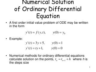
LECTURE-1INTRODUCTION • There exists large number of ordinary differential equations, whose solution cannot be obtained by the known analytical methods. In such cases, we use numerical methods to get an approximate solution o f a given differential equation with given initial condition.
NUMERICAL DIFFERIATION • Consider an ordinary differential equation of first order and first degree of the form • dy/dx = f ( x,y ) ………(1) • with the intial condition y (x0 ) = y0 which is called initial value problem. • T0 find the solution of the initial value problem of the form (1) by numerical methods, we divide the interval (a,b) on whcich the solution is derived in finite number of sub- intervals by the points
LECTURE-2TAYLOR’S SERIES METHOD • Consider the first order differential equation • dy/dx = f ( x, y )……..(1) with initial conditions y (xo ) = y0 then expanding y (x ) i.e f(x) in a Taylor’s series at the point xo we get y ( xo + h ) = y (x0 ) + hy1(x0) + h2/ 2! Y11(x0)+……. Note : Taylor’s series method can be applied only when the various derivatives of f(x,y) exist and the value of f (x-x0) in the expansion of y = f(x) near x0 must be very small so that the series is convergent.
LECTURE-3PICARDS METHOD OF SUCCESSIVE APPROXIMATION • Consider the differential equation • dy/dx = f (x,y) with intial conditions • y(x0) = y0 then • The first approximation y1 is obtained by • y1 = y0 + f( x,y0 ) dx • The second approximation y2 is obtained by y2 = y1 + f (x,y1 ) dx
PICARDS APPROXIMATION METHOD • The third approximation of y3 is obtained y by y2 is given by • y3 = y0 + f(x,y2) dx……….and so on • ………………………………… • …………………………………. • yn = y0 + f (x,yn-1) dx • The process of iteration is stopped when any two values of iteration are approximately the same. • Note : When x is large , the convergence is slow.
LECTURE-4EULER’S METHOD • Consider the differential equation • dy/dx = f(x,y)………..(1) • With the initial conditions y(x0) = y0 • The first approximation of y1 is given by • y1 = y0 +h f (x0,,y0 ) • The second approximation of y2 is given by • y2 = y1 + h f ( x0 + h,y1)
EULER’S METHOD • The third approximation of y3 is given by • y3 = y2 + h f ( x0 + 2h,y2 ) • ……………………………… • …………………………….. • ……………………………... • yn = yn-1 + h f [ x0 + (n-1)h,yn-1 ] • This is Eulers method to find an appproximate solution of the given differential equation.
IMPORTANT NOTE • Note : In Euler’s method, we approximate the curve of solution by the tangent in each interval i.e by a sequence of short lines. Unless h is small there will be large error in yn . The sequence of lines may also deviate considerably from the curve of solution. The process is very slow and the value of h must be smaller to obtain accuracy reasonably.
LECTURE-5MODIFIED EULER’S METHOD • By using Euler’s method, first we have to find the value of y1 = y0 + hf(x0 , y0) • WORKING RULE • Modified Euler’s formula is given by • yik+1 = yk + h/2 [ f(xk ,yk) + f(xk+1,yk+1 • when i=1,y(0)k+1 can be calculated • from Euler’s method.
MODIFIED EULER’S METHOD • When k=o,1,2,3,……..gives number of iterations • i = 1,2,3,…….gives number of times a particular iteration k is repeated when • i=1 • Y1k+1= yk + h/2 [ f(xk,yk) + f(xk+1,y k+1)],,,,,,
LECTURE-6RUNGE-KUTTA METHOD The basic advantage of using the Taylor series method lies in the calculation of higher order total derivatives of y. Euler’s method requires the smallness of h for attaining reasonable accuracy. In order to overcomes these disadvantages, the Runge-Kutta methods are designed to obtain greater accuracy and at the same time to avoid the need for calculating higher order derivatives.The advantage of these methods is that the functional values only required at some selected points on the subinterval.
R-K METHOD • Consider the differential equation • dy/dx = f ( x, y ) • With the initial conditions y (xo) = y0 • First order R-K method : • y1= y (x0 + h ) • Expanding by Taylor’s series • y1 = y0 +h y10 + h2/2 y110 +…….
LECTURE-7R-K METHOD • Also by Euler’s method • y1 = y0 + h f (x0 ,y0) • = y0 + h y10 • It follows that the Euler’s method agrees with the Taylor’s series solution upto the term in h. Hence, Euler’s method is the Runge-Kutta method of the first order.
The second order R-K method is given by • y1= y0 + ½ ( k1 + k2 ) • where k1 = h f ( x0,, y0 ) • k2 = h f (x0 + h ,y0 + k1 )
Third order R-K method is given by • y1 = y0 + 1/6 ( k1 + k2+ k3 ) • where k1 = h f ( x0 , y0 ) • k2 = hf(x0 +1/2h , y0 + ½ k1 ) • k3 =hf(x0 + ½h , y0 + ½ k2)
The Fourth order R – K method : This method is most commonly used and is often referred to as Runge – Kutta method only. Proceeding as mentioned above with local discretisation error in this method being O (h5), the increment K of y correspoding to an increment h of x by Runge – Kutta method from dy/dx = f(x,y),y(x0)=Y0 is given by
K1 = h f ( x0 , y0 ) • k2 = h f ( x0 + ½ h, y0 + ½ k1 ) • k3 = h f ( x0 + ½ h, y0 + ½ k2 ) • k4 = h f ( x0 + ½ h, y0 + ½ k3 ) • and finally computing • k = 1/6 ( k1 +2 k2 +2 k3 +k4 ) • Which gives the required approximate value as • y1 = y0 + k
R-K METHOD Note 1 : k is known as weighted mean of k1, k2, k3 and k4. Note 2 : The advantage of these methods is that the operation is identical whether the differential equation is linear or non-linear.
LECTURE-8PREDICTOR-CORRECTOR METHODS • We have discussed so far the methods in which a differential equation over an interval can be solved if the value of y only is known at the beginning of the interval. But, in the Predictor-Corrector method, four prior values are needed for finding the value of y at xk. • The advantage of these methods is to estimate error from successive approximations to yk
PREDICTOR-CORRECTOR METHOD • If xk and xk+1 be two consecutive points, such that xk+1=xk+h, then • Euler’s method is • Yk+1 = yk + hf(x0 +kh,yk) ,k= 0,1,2,3……. • First we estimate yk+1 and then this value of yk+1 is substituted to get a better approximation of y k+1.
LECTURE-9MILNE’S METHOD • This procedure is repeated till two consecutive iterated values of yk+1 are approximately equal. This technique of refining an initially crude estimate of yk+1 by means of a more accurate formula is known as Predictor- Corrector method. • Therefore, the equation is called the Predictor while the equation serves as a corrector of yk+1.Two such methods, namely, Adams- Moulton and Milne’s method are discussed.
MILNE’S METHOD • Consider the differntial equation • dy/dx = f ( x, y ), f (0 ) = 0 • Milne’s predictor formula is given by • Y(p)n+1=yn-3+4h/3(2y1n-y1n-1+2y1n-2) • Error estimates • E (p) = 28/29h5 yv
MILNE’S METHOD • The Milnes corrector formula is givenby • y(c)n+1=yn-1+h/3(y1n+1+4y1n+y1n-1) • The superscript c indicates that the value obtained is the corrected value and the superscript p on the right indicates that the predicted value of yn+1 should be used for computing the value of • f ( xn+1 , yn+1 ).
LECTURE-10ADAMS – MOULTON METHOD • Consider the differential equation • dy/dx = f ( x,y ), y(x0) = y0 • The Adams Moulton predictor formula is given by • y(p)n+1 = yn + h/24 [55y1n-59y1n-1+37y1n-2- 9y1n-3]
ADAM’S MOULTON METHOD • Adams – Moulton corrector formula is given by • Yn+1=yn+h/24[9y1pn+1 +19y1n-5-y1n-1+y1n-2] Error estimates EAB = 251/720 h5