Download
1 / 45
450 likes | 565 Views
Equations-of-motion technique applied to quantum dot models. Slava Kashcheyevs Amnon Aharony Ora Entin-Wohlman. Thursday seminar at March 9, 2006. cond-mat/0511656 Phys. Rev. B 73 (2006). Paradigm: the Anderson model. Anderson (1961) – dilute magnetic alloys

E N D
Equations-of-motion technique applied to quantum dot models Slava Kashcheyevs Amnon Aharony Ora Entin-Wohlman Thursday seminar at March 9, 2006 cond-mat/0511656 Phys. Rev. B 73 (2006)
Paradigm: the Anderson model Anderson (1961) – dilute magnetic alloys Glazman&Raikh, Ng&Lee (1988) – quantum dots • Generalizations • Structured leads (“mesoscopic network”) • Multilevel dots / multiple dots with capacitative / tunneling interactions • Spin-orbit interactions • Essential: many-body interactions restricted to the dot
How to treat Anderson model? • Perturbation theory (PT) in Γ, in U • analytic • controllable • tricky to extend into strong coupling (Kondo) regime • Map to a spinmodel and do scaling • Numerical Renormalization Group (NRG) • accurate low energy physics • inherently numerical • Bethe ansatz • exact analytic solution • integrability condition too restrictive, finite T laborious • Equations of motion(EOM) • analytic • as good as PT when PT is valid • not controlled for Kondo, but can give reasonable answers
Outline • Get equations • Definitions and the exact EOM hierarchy • Truncation: self-consistent vs. perturbative • Solve equations • Analysis of sum rules => bad news • Exact solution for => some good news • Kondo physics with EOM • pro and con
grand canonical Green’s functions Zubarev (1960) • Retarded • Advanced • Spectral function
Equations of motion Green function on the dot
fully characterizes the leads Γ D Wide-band limit: – approximate Green function in simple cases • No interactions (U=0)
Green function in simple cases • Small U – approximate the extra term Strict 1st order Self-consistent (Hartree) Decouple via Wick Expand to 1st order Anderson (1961)
m = 0,1, 2… lead operators n = 0 – 3 dot operators General term in the EOM • increases the total number of operators by adding two extra d’s • Not more than can accumulate on the lhs of GF (finite Hilbert space on the dot!) • Vk transforms d’s into lead c’s that do accumulate Contributes to a least m-th order in Vkand (n+m–1)/2-th order in U ! Dworin (1967)
spin conservation • Use values Meir, Wigreen, Lee(1991) Decoupling “D.C.Mattis scheme”: Theumann (1969) • Stop before we get 6 operator functions
Meir-Wingreen –Lee (1991) • Well characterizes Coulomb blockade downs to T ~ Γ • Popular and easy to use • Would be exact to , if one treated to 1st order • Often referred to as “…works quantitatively at T > TK, and qualitatively at T< TK” – a misleading statement
spin conservation • Use values Meir, Wigreen, Lee(1991) • Demand full self-consistency Appelbaum&Penn (1969); Lacroix(1981) Entin,Aharony,Meir (2005) Decoupling “D.C.Mattis scheme”: Theumann (1969) • Stop before we get 6 operator functions
Self-consistent equations Self-consistent functions: Zeeman splitting Level position The only input parameters
Outline • Get equations • Definitions and the exact EOM hierarchy • Truncation: self-consistent vs. perturbative • Solve equations • Analysis of sum rules => bad news • Exact solution for => some good news • Kondo physics with EOM • pro and con
First test: the sum rules Langreth (1966) • Relations at T=0 and Fermi energy: • MWL approach gives . Will self-consistency improve this? 0 “Unitarity” condition Friedel sum rule (For simplicity, look at the wide band limit )
P and Q develop logarithmic singularities at T=0 as when either of these is 0, will have an equation for Exploit low T singularities Integration with the Fermi function: T=0
Results for the sum rules • Expected: • For and • For and “Unitarity” is OK “Unitarity” is OK Friedel implies: Field-independent magnetization !
middle of Coulomb blockade valley no Zeeman splitting symmetric band Particle-hole symmetry • This implies symmetric DOS: Exact cancellation in numerator & denominator separately at any T!
Particle-hole symmetry • Temperature-independent (!) Green function • At T=0 the “unitarity” rule is broken: • The problem is mentioned in Dworin (1967), Appelbaum&Penn (1969), but in no paper after 1970! • The Green function of Meir, Wingreen & Lee (1991) gives the same
“Unitarity” Friedel T In this plane, and limits do not commute Sum rules: summary T=0 plane “Unitarity” Friedel (“softly”) “Unitarity” Friedel ?
Ouline • Get equations • Definitions and the exact EOM hierarchy • Truncation: self-consistent vs. perturbative • Solve equations • Analysis of sum rules => bad news • Exact solution for => some good news • Kondo physics with EOM • pro and con
remove integration remove non-linearity Exactly solvable limit • Requires and wide-band limit • Explicit quadrature expression for the Green function • Self-consistency equation for 3 numbers (occupation numbers and a parameter) • Will show how to …. Skip to Results...
Retarded couples to advanced and vice versa Infinite U limit + wide band A known function:
How to get rid of integration? • Can we write the equations as algebraic relations between functions defined on the upper and lower edges of the cut? Does not work for the unknown function:
How to get rid of integration? • Introduce two new unknown functions Φ1 and Φ2 (linear combinations of P and I), • and two known X1 and X2 such that:
Cancellation of non-linearity Clear fractions and add: • The function must be a polynomial! • Considering gives ,where r0 and r1 are certain integrals of the unknown Green function
From asymptotics, Explicit solution! Riemann-Hilbert problem • Remain with 2 decoupled linear problems: A polynomial! • Expanding for large z gives a set of equations for a1, r0, r1 and <nd> • The retarded Green function is given by
Outline • Get equations • Definitions and the exact EOM hierarchy • Truncation: self-consistent vs. perturbative • Solve equations • Analysis of sum rules => bad news • Exact solution for => some good news • Kondo physics with EOM • pro and con
Ed / Γ Energy ω/Γ Fermi Results: density of states • Zero temperature • Zero magnetic field • & wide band Level renormalization Changing Ed/Γ Looking at DOS:
Results: occupation numbers • Compare to perturbation theory • Compare to Bethe ansatz Gefen & Kőnig (2005) Wiegmann & Tsvelik (1983) Better than 3% accuracy!
Results: Friedel sum rule Good – for nearly empty dot Broken – in the Kondo valley • “Unitarity” sum rule is fulfilled exactly: • Use Friedel sum rule to calculate
2e2/h conduct. ~ 1/log2(T/TK) Results: Kondo peak melting At small T and near Fermi energy, parameters in the solution combine as Smaller than the true Kondo T: DOS at the Fermi energy scales with T/TK*
Magnetic susceptibility • Defined as • Explicit formula obtained by differentiating equations for with respect to h. χ Wide-band limit
Bethe susceptibility in the Kondo regime ~1/TK Our χ is smaller, but on the other hand TK*<<TK ?! Results: magnetic susceptibility !
TK* Γ Results: susceptibility vs. T
Results: MWL susceptibility MWL gives non-monotonic and even negative χ for T < Γ
Conclusions! • EOM is a systematic method to derive analytic expressions for GF • Wise (sometimes) extrapolation of perturbation theory • Applied to Anderson model, • excellent for not-too-strong correlations • fair qualitative picture of the Kondo regime • self-consistency improves a lot
Thanks! Paper, poster & talk atkashcheyevs