Another Take on Patch-Based Image Processing
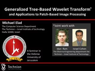
*. Another Take on Patch-Based Image Processing . Michael Elad The Computer Science Department The Technion – Israel Institute of technology Haifa 32000, Israel. *Joint work with Idan Ram Israel Cohen

Another Take on Patch-Based Image Processing
E N D
Presentation Transcript
* Another Take on Patch-Based Image Processing Michael Elad The Computer Science Department The Technion – Israel Institute of technology Haifa 32000, Israel *Joint work with Idan Ram Israel Cohen The Electrical Engineering department Technion – Israel Institute of Technology Workshop SIGMA'2012 SIGNAL, IMAGE, GEOMETRY, MODELLING, APPROXIMATION
Patch-Based Processing of Images In the past decade we see more and more researchers suggesting to process a signal or an image with a paradigm of the form: Break the given image into overlapping (small) patches Operate on the patches separately or by exploiting inter-relation between them Put back the resulting patches into a result canvas 2
Patch-Based Processing of Images In the past decade we see more and more researchers suggesting to process a signal or an image with a paradigm of the form: Surprisingly, these methods are very effective, actually leading to today’s state-of-the-art in many applications Common theme: The image patches are believed to exhibit a highly-structured geometrical form in the embedding space they reside in 3
Patches … Patches … Patches … Who are the researchers promoting this line of work? Many leading scientists from various places Various Ideas: Non-local-means Kernel regression Sparse representations Locally-learned dictionaries BM3D Structured sparsity Structural clustering Subspace clustering Gaussian-mixture-models Non-local sparse rep. Self-similarity Manifold learning … You Sorry if I forgot YOU & … You? 4
This Talk is About … A different way to treat an image using its overlapped patches Order to form the shortest possible path Process the Patches 5
Surprisingly, This Talk is Also About … Processing of Non-Conventionally Structured Signals Many signal-processing tools (filters, transforms, …) are tailored for uniformly sampled signals Now we encounter different types of signals: e.g., point-clouds and graphs. Can we extend classical tools to these signals? Our goal: Generalize the wavelet transform to handle this broad family of signals In the process, we will find ourselves returning to “regular” signals, handling them differently In fact, this is how this work started in the first place 6
Part I – GTBWT Generalized Tree-Based Wavelet Transform – The Basics This part is taken from the following two papers: • I. Ram, M. Elad, and I. Cohen, “Generalized Tree-Based Wavelet Transform”, IEEE Trans. Signal Processing, vol. 59, no. 9, pp. 4199–4209, 2011. • I. Ram, M. Elad, and I. Cohen, “Redundant Wavelets on Graphs and High Dimensional Data Clouds”, IEEE Signal Processing Letters, Vol. 19, No. 5, pp. 291–294 , May 2012. 7
Problem Formulation • We start with a set of points . These could be • Feature points associated with the nodes of a graph. • Set of coordinates for a point-cloud in high-dimensional space. • A scalar function is defined on these coordinates, , our signal to process is . • We may regard this dataset as a set of samples taken from a high-dimensional function . • Key assumption – A distance-measure between points in is available to us. The function behind the scene is “regular”: … … Small implies small for almost every pair 8
Our Goal Sparse (compact) Representation Wavelet Transform • We develop both an orthogonal wavelet transform and a redundant alternative, both efficiently representing the input signal f. • Our problem: The regular wavelet transform produces a small number of large coefficients when it is applied to piecewise regular signals. But, the signal (vector) f is not necessarily smooth in general. 9
Previous and Related Work “Diffusion Wavelets” R. R. Coifman, and M. Maggioni, 2006. “Multiscale Methods for Data on Graphs and Irregular Multidimensional Situations” M. Jansen, G. P. Nason, and B. W. Silverman, 2008. “Wavelets on Graph via SpectalGraph Theory” D. K. Hammond, and P. Vandergheynst, and R. Gribonval, 2010. “Multiscale Wavelets on Trees, Graphs and High Dimensional Data: Theory and Applications to Semi Supervised Learning” M . Gavish, and B. Nadler, and R. R. Coifman, 2010. “Wavelet Shrinkage on Paths for Denoising of Scattered Data” D. Heinen and G. Plonka, to appear 10
The Main Idea (1) - Permutation Permutation using Permutation 1D Wavelet P T T-1 P-1 Processing 11
The Main Idea (2) - Permutation • In fact, we propose to perform a differentpermutation in each resolution level of the multi-scale pyramid: • Naturally, these permutations will be applied reversely in the inverse transform. • Thus, the difference between this and the plain 1D wavelet transform applied on f are the additional permutations, thus preserving the transform’s linearity and unitarity, while also adapting to the input signal. 12
250 250 200 200 150 150 100 100 50 50 0 0 0 50 100 150 200 250 0 50 100 150 200 250 Building the Permutations (1) • Lets start with P0 – the permutation applied on the incoming signal. • Recall: the wavelet transform is most effective for piecewise regular signals. → thus, P0 should be chosen such that P0f is most “regular”. • So, … for example, we can simply permute by sorting the signal f… 13
Building the Permutations (2) • However: we will be dealing with corrupted signals f (noisy, missing values, …) and thus such a sort operation is impossible. • To our help comes the feature vectors in X, which reflect on the order of the signal values, fk. Recall: • Thus, instead of solving for the optimal permutation that “simplifies” f, we order the features in X to the shortest path that visits in each point once, in what will be an instance of the Traveling-Salesman-Problem (TSP): Small implies small for almost every pair 14
Building the Permutations (3) • We handle the TSP task by a simple (and crude) approximation: • Initialize with an arbitrary index j; • Initialize the set of chosen indices to Ω(1)={j}; • Repeat k=1:1:N-1 times: • Find xi– the nearest neighbor to xΩ(k) such that iΩ; • Set Ω(k+1)={i}; • Result: the set Ωholds the proposed ordering. 15
Building the Permutations (4) • So far we concentrated on P0 at the finest level of the multi-scale pyramid. • In order to construct P1, P2, … ,PL-1, the permutations at the other pyramid’s levels, we use the same method, applied on propagated (reordered, filtered and sub-sampled) feature-vectors through the same wavelet pyramid: P1 P0 LP-Filtering (h) & Sub-sampling LP-Filtering (h) & Sub-sampling P3 LP-Filtering (h) & Sub-sampling P2 LP-Filtering (h) & Sub-sampling 16
Why “Generalized Tree …”? • “Generalized” tree Tree (Haar wavelet) • Our proposed transform: Generalized Tree-Based Wavelet Transform (GTBWT). • We also developed a redundant version of this transform based on the stationary wavelet transform [Shensa, 1992][Beylkin, 1992]– also related to the “A-TrousWavelet” (will not be presented here). • At this stage we could (or should) show how this works on point clouds/graphs, but we will take a different route and demonstrate these tools for images. 17
Part II – Handling Images Using GTBWT by Handling Image Patches This part is taken from the same papers mentioned before … • I. Ram, M. Elad, and I. Cohen, “Generalized Tree-Based Wavelet Transform”, IEEE Trans. Signal Processing, vol. 59, no. 9, pp. 4199–4209, 2011. • I. Ram, M. Elad, and I. Cohen, “Redundant Wavelets on Graphs and High Dimensional Data Clouds”, IEEE Signal Processing Letters, Vol. 19, No. 5, pp. 291–294 , May 2012. 18
Could Images Fit This Data-Structure? • Yes. Starting with an image of size do the following: • Extract all possible patches of size with complete overlaps – these will serve as the set of features (or coordinates) matrix X. • The values will be the center pixel in these patches. • Once constructed this way, we forget all about spatial proximities in the image , and start thinking in terms of (Euclidean) proximities between patches. * * Not exactly. Actually, if we search the nearest-neighbors within a limited window, some of the spatial proximity remains. 19
55 50 45 40 35 PSNR 30 25 20 15 10 0 2000 4000 6000 8000 10000 # Coefficients Lets Try (1) • For a 128×128 center portion of the image Lenna, we compare the image representation efficiency of the • GTBWT • A common 1D wavelet transform • 2D wavelet transform. • We measure efficiency by the m-term approximation error, i.e. reconstructing the image from m largest coefficients, zeroing the rest. GTBWT – permutation at the finest level 2D common 1D db4 20
55 50 45 40 35 PSNR 30 25 20 15 10 0 2000 4000 6000 8000 10000 # Coefficients Lets Try (2) • For a 128×128 center portion of the image Lenna, we compare the image representation efficiency of the • GTBWT • A common 1D wavelet transform • 2D wavelet transform. • We measure efficiency by the m-term approximation error, i.e. reconstructing the image from m largest coefficients, zeroing the rest. GTBWT – permutations at the finest two level 2D common 1D common 1D db4 db4 21
55 50 45 40 35 PSNR 30 25 20 15 10 0 2000 4000 6000 8000 10000 # Coefficients Lets Try (3) • For a 128×128 center portion of the image Lenna, we compare the image representation efficiency of the • GTBWT • A common 1D wavelet transform • 2D wavelet transform. • We measure efficiency by the m-term approximation error, i.e. reconstructing the image from m largest coefficients, zeroing the rest. GTBWT – permutations at the finest three level 2D common 1D db4 22
55 50 45 40 35 PSNR 30 25 20 15 10 0 2000 4000 6000 8000 10000 # Coefficients Lets Try (4) • For a 128×128 center portion of the image Lenna, we compare the image representation efficiency of the • GTBWT • A common 1D wavelet transform • 2D wavelet transform. • We measure efficiency by the m-term approximation error, i.e. reconstructing the image from m largest coefficients, zeroing the rest. GTBWT – permutations at all (10) levels 2D common 1D db4 23
Comparison Between Different Wavelets db1 (Haar) db4 GTBWT comparison db8 24
The Representation’s Atoms – Synthetic Image wavelets wavelets wavelets wavelets wavelets Scaling functions Original image wavelets wavelets wavelets wavelets wavelets wavelets wavelets 25
The Representation’s Atoms – Lenna wavelets wavelets wavelets wavelets Scaling functions Original image wavelets wavelets wavelets wavelets wavelets wavelets 26
Image Denoising using GTBWT • We assume that the noisy image, , is a noisy version of a clean image, , contaminated by white zero-mean Gaussian additive noise with known STD=. • The vectors and are lexicographic ordering of the noisy and clean images. • Our goal: recover from , and we will do this using shrinkage over GTBWT: • We extract all patches from the noisy image as described above; • We apply the GTBWT on this data set; • The wavelet coefficients obtained go through a shrinkage operation; and • We transform back to get the final outcome. 27
Image Denoising – Block-Diagram Noisy image GTBWT Reconstructed image Hard thresholding (GTBWT)-1 28
Image Denoising – Improvements Cycle-spinning: Apply the above scheme several (10) times, with a different GTBWT (different random ordering), and average. Noisy image Reconstructed image GTBWT-1 GTBWT-1 THR Averaging THR GTBWT GTBWT 29
Image Denoising – Improvements Sub-image averaging: A by-product of GTBWT is the propagation of the whole patches. Thus, we get n transform vectors, each for a shifted version of the image and those can be averaged. P0 LP-Filtering (h) & Sub-sampling P1 LP-Filtering (h) & Sub-sampling HP-Filtering (g) & Sub-sampling HP-Filtering (g) & Sub-sampling P3 LP-Filtering (h) & Sub-sampling P2 LP-Filtering (h) & Sub-sampling HP-Filtering (g) & Sub-sampling HP-Filtering (g) & Sub-sampling 30
Image Denoising – Improvements • Sub-image averaging: A by-product of GTBWT is the propagation of the whole patches. Thus, we get n transform vectors, each for a shifted version of the image and those can be averaged. • Combine these transformed pieces; • The center row is the transformed coefficients of f. • The other rows are also transform coefficients – of n shifted versions of the image. • We can reconstruct n versions of the image and average. P0 LP-Filtering (h) & Sub-sampling P1 LP-Filtering (h) & Sub-sampling HP-Filtering (g) & Sub-sampling HP-Filtering (g) & Sub-sampling P3 LP-Filtering (h) & Sub-sampling P2 LP-Filtering (h) & Sub-sampling HP-Filtering (g) & Sub-sampling HP-Filtering (g) & Sub-sampling 31
Image Denoising – Improvements Restricting the NN: It appears that when searching the nearest-neighbor for the ordering, restriction to near-by area is helpful, both computationally (obviously) and in terms of the output quality. Patch of size Search-Area of size 32
Image Denoising – Improvements • Improved thresholding: Instead of thresholding the wavelet coefficients based on their value, threshold them based on the norm of the (transformed) vector they belong to: • Recall the transformed vectors as described earlier. • Classical thresholding: every coefficient within is passed through the function: • The proposed alternative would be to force “joint-sparsity” on the above array of coefficients, forcing all rows to share the same support: 33
Image Denoising – Results • We apply the proposed scheme with the Symmlet 8 wavelet to noisy versions of the images Lena and Barbara • For comparison reasons, we also apply to the two images the K-SVD and BM3D algorithms. • The PSNR results are quite good and competitive. • What about run time? 34
Relation to BM3D? Our scheme BM3D 3D Transform & threshold In a nut-shell, while BM3D searches for patch neighbors and process them locally, our approach seeks one path through all the patches (each gets its own neighbors as a consequence), and the eventual processing is done globally. 3D Transform & threshold Reorder, GTBWT, and threshold 35
Part III – Frame Interpreting the GTBWT as a Frame and using it as a Regularizer This part is documented in the following draft: • I. Ram, M. Elad, and I. Cohen, “The RTBWT Frame – Theory and Use for Images”, working draft to be submitted soon. We rely heavily on • Danielyan, Katkovnik, and Eigiazarian, “BM3D frames and Variational Image Deblurring”, IEEE Trans. on Image Processing, Vol. 21, No. 4, pp. 1715-1728, April 2012. 36
Recall Our Core Scheme Reconstructed image GTBWT Noisy image Hard Thresholding Or, put differently, : We refer to GTBWT as a redundant frame, and use a “heuristic” shrinkage method with it, which aims to approximate the solution of Synthesis: or Analysis: (GTBWT)-1 37
So, Who is Our Frame? Bottom line: The redundancy of our frame is 64J P0 LP-Filtering (h) & Sub-sampling Array of overlapped patches of size* 64N We obtain an array of 64JN transform coefficients P3 LP-Filtering (h) & Sub-sampling P2 LP-Filtering (h) & Sub-sampling P1 LP-Filtering (h) & Sub-sampling HP-Filtering (g) & Sub-sampling HP-Filtering (g) & Sub-sampling Applying a J redundant wavelet of some sort with permutations Lexicographic ordering of the N pixels * For patches of size 8×8 pixels HP-Filtering (g) & Sub-sampling HP-Filtering (g) & Sub-sampling 38
What Can We Do With This Frame? • We could solve various inverse problems of the form: • where: x is the original image • v is an AWGN, and • A is a degradation operator of any sort • We could consider the synthesis, the analysis, or their combination: 40
Generalized Nash Equilibrium * Instead of minimizing the joint analysis/synthesis problem: break it down into two separate and easy to handle parts: and solve iteratively * Danielyan, Katkovnik, and Eigiazarian, “BM3D frames and Variational Image Deblurring”, IEEE Trans. on Image Processing, Vol. 21, No. 4, pp. 1715-1728, April 2012. 41
Deblurring Results Original Blurred Restored 42
Deblurring Results Blur PSF = 2=2 43
Part IV – Patch (Re)-Ordering Lets Simplify Things, Shall We? This part is based on the paper: • I. Ram, M. Elad, and I. Cohen, “Image Processing using Smooth Ordering of its Patches”, Submitted to IEEE Transactions on Image Processing. 44
Returning to the Basics Then we order these patches to form the shortest path, as before We extract all (with overlaps) patches of size B×B (e.g. B=20) Suppose we start with a clean image What should we expect? 45
Spatial Neighbor Euclidean Neighbor Spatial neighbors are not necessarily expected to remain neighbors in the new ordering 0 10 Peppers Barbara -1 10 -2 Histogram 10 -3 10 -4 10 What should we expect? 0 100 200 300 400 Sqrt Euclidean Distance 46
The Reordered Signal is More Regular What should we expect? Considering the center (or any other) pixel in each patch, the new path is expected to lead to very smooth (or at least, piece-wise smooth) 1D signal. * * Measure of smoothness: Raster scan: 9.57 Hilbert curve: 11.77 Sorted (ours): 5.63 47
Processing the Permuted Pixels • Assumptions: • After a shortest-path reordering of the patches form a clean image, we expect a highly regular signal. • Reordering a corrupted image is likely to lead to a good quality sort, due to the robustness brought by the patch-matching. An Idea: Given a corrupted image of the form: where: x is the original image v is an AWGN, and M is a point-wise degradation operator, Apply this process: Re-order the pixels to a 1D signal Re-order the pixels back to their location Process the 1D signal with a simple filter Corrupted Image 48
Use the Reordering for Denoising Noisy with =25 (20.18dB) * This result is obtained with (i) cycle-spinning, (ii) sub-image averaging, (iii) two iterations, (iv) learning the filter , and (v) switched smoothing. Order these patches as before (TSP) Extract all (with overlaps) patches of size 10×10 Reconstruction: 32.65dB * Take the center-row – it represents a permutation of the image pixels to a regular function Smooth/filter the values along this row in a simple way 49
Intuition: Why Should This Work? True samples Noisy samples Noisy with =25 (20.18dB) Ordering based on the noisy pixels Reconstruction: 32.65dB Simple smoothing 50