Download
1 / 44
440 likes | 463 Views
Ph.D. COURSE IN BIOSTATISTICS DAY 6. A BRIEF REVIEW OF BASIC FACTS ABOUT STATISTICAL METHODS BASED ON LIKELIHOOD FUNCTIONS. The normal distribution and the binomial distribution are examples of parametric statistical models.

E N D
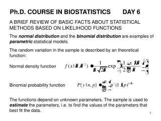
Ph.D. COURSE IN BIOSTATISTICS DAY 6 A BRIEF REVIEW OF BASIC FACTS ABOUT STATISTICAL METHODS BASED ON LIKELIHOOD FUNCTIONS The normal distribution and the binomial distribution are examples of parametric statistical models. The random variation in the sample is described by an theoretical function: Normal density function Binomial probability function The functions depend on unknown parameters. The sample is used to estimate the parameters, i.e. to find the values of the parameters that best fit the data.
Example: Change in diastolic blood pressure in pregnant women (lectures, day 2, page 11) A histogram of the data in the control group and the best fitting normal distribution The best fitting normal distribution was determined as the normal distribution with excepted value equal to the sample average and variance equal to the sample variance. Intuitively reasonable.
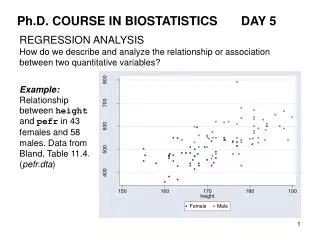
Example: Estimation of the 2-years survival probability in a clinical trial (lectures, day 4, page 7) Data on 88 patients, 35 died within the first two years of follow-up. The number of deaths was described by a binomial distribution with probability parameter equal to the relative frequency of death. Again, intuitively reasonable. Example:Linear regression of pefr on height (lectures, day 5, page 1) Data on pefr and height from 43 females and 58 males were described as points scattered around a straight line (line regression model). The estimates of intercept and slope were determined by the methods of least squares. The method has some intuitive appeal, but the estimates are not obvious. What to do in general ? For more complicated models, e.g. logistic regression, it is not obvious how to obtain good estimates – and what do we mean by “good”?
THE MAXIMUM LIKELIHOOD METHOD We need a general method of estimation which give estimates with good – preferably optimal – properties. The maximum likelihood method is such a method. Likelihood function = Function of the parameters which for each value of the parameter(s) gives the probability of observing the data. Maximum likelihood estimation: Choose the value of the parameter(s) which maximize the likelihood function, i.e. the value(s) which make the probability of observing the actual data as large as possible. Note: The estimation problem is now reformulated as a mathematical problem of finding the maximum of a function of one or several parameters. The solution to this problem is well-known (high school calculus): Compute the first derivative of the function with respect to the parameter and find the value for which the first derivative is 0, etc.
The maximum likelihood method has some intuitive appeal: The dataThe crime The parameters The suspects The maximum likelihood The suspects whose probability of estimate having committed the crime is largest Note: P{ crime | suspect } is not the same as P{ suspects | crime } Example: one-sample problem with dichotomous response Data: A sample of size n of failures (0) and successes (1), e.g. We have where
The likelihood function therefore becomes Maximizing the likelihood function is equivalent to maximizing the logarithm of the likelihood function, and the later is easier.
The first derivative of the log-likelihood function The maximum-likelihood estimate is found as the solution to A little algebra shows that the solution is The solution is a maximum since the second derivative is negative If the random variation is described by a normal distribution the maximum likelihood method is equivalent to the method of least squares, so the estimates of intercept and slope in a linear regression model are also maximum likelihood estimates.
IS THIS A GOOD METHOD? If the model is correctly specified it can be shown (under suitable regularity conditions) that 1. The maximum likelihood estimate will approach the true value as the sample size increases. 2. For large sample sizes the random error of the estimate is approximately normal 3. No other estimate having properties 1. and 2. has smaller standard error 4. All (almost) the usual estimates are maximum likelihood estimates Property 1 shows that maximum-likelihood estimates are asymptotically unbiased. Property 2 ensures that in large sample confidence intervals can be computed as estimate ± 1.96·se(estimate). Property 3 shows that the estimates are optimal.
STANDARD ERRORS OF ESTIMATES Intuitively, the imprecision of the maximum likelihood estimate is related to the “flatness” of the log-likelihood function at its maximum. The “flatness” is measured by the curvature, the second derivative, which describes the change in the slope of the tangent to the curve. If e.g. the curve is flat the second derivative is small. This suggests that the uncertainty in the estimate is inversely related to the second derivative of the log-likelihood function. Exampleone-sample problem with dichotomous response - continued Here we have At the maximum we find
In this example an estimate of the standard error of the estimate satisfies This result is not restricted to the simple model considered here, but holds quite generally, and therefore gives an method to obtain (approximate) standard errors of maximum-likelihood estimates. The uncertainty in the maximum-likelihood estimate is approximately normal in large samples, and the result shows that approximate 95% confidence intervals can be obtained as estimate ± 1.96·se(estimate), where the standard error is obtained from expression of the form above. In the example the statistical model had only a single unknown parameter. Analogous results are available for multi-parameter problems. When Stata in complicated regression models gives parameter estimates with estimated standard errors, these estimates are computed from general results for multi-parameter models.
TEST OF HYPOTHESES Consider a statistical model depending on a single parameter . The maximum likelihood estimate is the parameter value which maximizes Hypothesis: Idea: Consider the ratio We obviously have Q is close to 1: The value describes the data almost as well as the best choice, i.e. the hypothesis is consistent with the data. Q is close to 0: The probability of observing the data when is much smaller than the maximum probability, i.e. other values of the parameter describes the data much better. The hypothesis is therefore not supported by the data.
The test statistic Q is called the likelihood ratio test. Mathematical result For large samples the distribution of is approximately a -distribution with 1 degree of freedom is the hypothesis is true. Large values of the deviance corresponds to small values of Q and therefore provide evidence against the hypothesis. Asymptotically equivalent test statistics: The Score test: Wald’s test: The test statistics S and W are also approximately -distributed with 1 degree of freedom if the null hypothesis is true.
In large samples the three test statistics will yield essentially identical results Analogous results are available for multi-parameter problems. For a specific problem one or the other test statistic may be easier to compute. Many of the well-known statistical test can be shown to be either a Score test or a Wald’s test. The usual X2-testof independence inan R×C table is e.g. a Score test. Statistical programs like Stata and SPSS will usually compute one or several of these test statistics. Confidence intervals again A confidence interval is defined as the parameter values that are not statistically significant. Since there are several equivalent test statistics, there are also several versions of (approximate) confidence intervals. The confidence intervals based on Wald’s test have the familiar form: estimate ± 1.96·se(estimate). Confidence intervals based on the deviance are believe to be slightly more accurate, but are more complex to compute and therefore not always included in Statistical packages.
COMPUTING SAMPLE SIZE AND STATISTICAL POWER In the planning of an investigation the size of the study has to be determined. Statistical considerations relevant for the decision is considered here. Two main types of situations • Sample size determined to obtain a required precision of an estimate. • Mainly relevant when the purpose is to estimate a certain aspect of • the population. • Sample size determined to obtain a given power against a specified • alternative. • Mainly relevant in comparative studies. Also relevant to turn the problem around and compute precision or power for a given sample size to see if a planned study is likely to produce useful results.
Re. 1. Sample size to meet a required precision. The standard error of an estimate is usually inversely proportional to the square-root of the sample size The width of an approximate 95% confidence interval is roughly four times the standard error. The sample size necessary to give a confidence interval of a given width, w, is therefore approximately For an average For a proportion To use these formulas preliminary estimates of or pmust be inserted in the right hand side of formulas. The approach is readily extended to other estimates, e.g. the difference of two means or the slope of a regression line.
Re. 2. Sample size to meet a required power for a specified alternative. To identify the basic issues consider the following simple situation: Data: We plan to collect a random sample from a normal population with mean and standard deviation . Purpose: We want to assess the hypothesis in such a way that if the true value is actually , then the hypothesis is rejected with a high probability. The test statistic has the form (assuming that is known) If the level of significance is 5% the hypothesis is not rejected when This interval is called the acceptance region of the test.
The level of significance, usually denoted , specifies the risk of rejecting of true hypothesis. This is called the risk of Type 1 error. Now, suppose that the alternative value is the true value. The correct decision is then to reject the hypothesis . The probability of correctly rejecting the hypothesis if the is called the power of the statistical test. The probability of not rejecting a false hypothesis is called the risk of Type 2 error and is usually denoted . Power + Risk of Type 2 error = 1 Note that the power depends on the value , so it does not make sense to talk about power or risk of Type 2 error without specifying the alternative value for which they are computed. In a sample size calculation we find the minimum sample size for which the the statistical test has a given power for a specified alternative. For a given sample size we may alternatively find the power of the test for a specified alternative.
Illustration of basic concepts Blue line indicates the acceptance region Black curve shows the distribution of the mean when Red curve shows the distribution of the mean when The power of the test is the area under the red curve outside the acceptance region. Note: A contribution from each tail, but one of them can usually be ignored.
The simple situation: Formulas for sample size and power Notation Level of significance (risk of Type 1 error) Risk of Type 2 error = 1 – Power Standard normal variate: Standard normal percentiles Minimum sample size for given power the first factor becomes 7.85 the first factor becomes 10.5 Power for given sample size
DETERMINING SAMPLE SIZE FOR TWO SAMPLE PROBLEMS Setting: A randomized clinical trial to compare two treatments, a standard treatment and a new treatment. Basic problem: How large should the trial be? • Questions that need to be answered first • What is the main purpose of the study? • What is the main response variable? • How should the data be analyzed? • What is the expected response with standard treatment? • How large is the random variation? • How small a difference between expected responses is it desirable • to detect and with what probability? Here comparison of two sample of (approximately) the same size with normal or binomial response.
A quantitative response variable that has a • normal distribution Notation Expected response with standard treatment Expected response with new treatment. The difference represents a treatment difference considered important to identify. The standard deviation of the response in each group (assumed to be the same in the two groups). Error probabilities as above The number of individuals in each group The total number of individuals in the study = 2n The sample of each group is given by
The factor depends only on the error probabilities Risk of Type 2 error Risk of Type 1 error Table of for selected values of Example Expected response in active drug group = 12 Expected response in placebo group = 4 Standard deviation = 10 level of significance = 0.05, power = 0.80 The total study size = N = 50
B. A dichotomous response variable (binomial frequencies) For each individual presence or absence of an event is recorded Notation Response probability with standard treatment Response probability with new treatment. The difference represents a treatment difference considered important to identify. Error probabilities as above The number of individuals in each group The total number of individuals in the study = 2n Many different formulas for the sample size is available. The following is simple and reasonably accurate. The sample of each group is given by same function as the one tabulated above
Example In a randomized clinical trial a new therapy is to be compared with the current standard therapy. The two-year survival probability with standard treatment is 0.60 Preliminary studies indicate that the survival probability with the new therapy is 0.70. If real, this improvement is so important that it should be identified with a high probability. Error probabilities are specified as Risk of Type 1 error = 0.05 Risk of Type 2 error = 0.10 Consequently, the trial should include in each treatment group, i.e. a total of 946 patients.
USING STATA FOR SAMPLE SIZE AND POWER CALCULATIONS Stata has a command, sampsi, which can be used for calculation of sample size and power for one- and two-sample problems. Two-sample problem with normal data. • To get the sample size calculation on page 22 write • sampsi 12 4 , sd1(10) power(0.80) Estimated sample size for two-sample comparison of means Test Ho: m1 = m2, where m1 is the mean in population 1 and m2 is the mean in population 2 Assumptions: alpha = 0.0500 (two-sided) power = 0.8000 m1 = 12 m2 = 4 sd1 = 10 sd2 = 10 n2/n1 = 1.00 Estimated required sample sizes: n1 = 25 n2 = 25 mean in sample 1 mean in sample 2
Options alpha(#) Level of significance. If omitted alpha(0.05) is assumed. power(#) Specifies the desired power. If omitted power(0.90) is assumed. sd1(#) Standard deviation in sample 1 sd2(#) Standard deviation in sample 2. If omitted a common value of the standard deviations are assumed. n1(#) Size of sample 1. If included power rather than sample size is computed. n2(#) Size of sample 2. If omitted the relation n2 = ratioxn1 is used. ratio(#) Ratio of sample sizes (= n2/n1). Used in conjuction with either n1(#) or n2(#). If omitted ratio(1) is assumed. onesample One-sample test. Default is two-sample test If neither sd1(#) nor sd2(#) is specified, sampsi assumes a test of proportions and the arguments are interpreted as proportion
Some examples • Two-sample test with normal data, unequal variance and ratio • of sample sizes equal to 2. Required sample size • sampsi 40 60 , sd1(10) sd2(20) ratio(2) • One-sample test with normal data, hypothesized value = 10, • alternative value = 20. Power calculation. • sampsi 10 20 , sd1(20) onesamplen1(40) • Two-sample test with dichotomous data. Required sample size • sampsi 0.6 0.7 The result is indicating that the simple approximation, which gave 473, is under-estimating the sample size slightly. • Two-sample test with dichotomous data and specified sample sizes. • Power calculation. • sampsi 0.08 0.05 , n1(500) n2(2000)
Example Suppose the mean birth weight of children born by no-smokers is 3.6 kg and by smokers it is 3.4 kg. Assume moreover that the standard deviation is 0.5 kg in both cases. The command sampsi 3.6 3.4 , sd1(.5) gives , the number of births that must be included in each sample if a statistical power of 0.90 is required. Now suppose that we decide not to analyze the actual weight, but only if the weight exceeds 3.5 kg. How large samples are then needed to get a power of 0.90? display 1-norm((3.5-3.6)/0.5) gives 0.57925971 display 1-norm((3.5-3.4)/0.5) gives 0.42074029 so the desired power is found by sampsi 0.5793 0.4207as The sample size has to be increased by 67% to account for the lost of information caused by replacing the actual weight by the dichotomous variable weight>3.5 kg.
COMMENTS The power and sample size calculations described here assume that the data are to be analyzed by either a t-test or a one- or two-sample test for analysis of proportions. Calculations based on non-parametric tests are complicated and is usually replaced by calculations based on normal distributions. This is justified by the fact that non-parametric tests are only slightly less powerful than normal theory counterparts. In large trials the data are often evaluated a couple of times during trial period, so-called interim analyses. This practice affects the error probabilities if not properly accounted for. Sample size and power calculations are often a useful part of the planning of a study. Once the data are collected a confidence interval for the parameter of interest is the most relevant way to express the precision (or lack of precision) of the study.
REVIEW AND ADVICE To improve the chance of making a relevant and satsfactory statistical analysis start by identifying the main purpose. Note that an analysis of a set of data usually should be divided in sub-analyses each with a specific purpose. • Description of the data • Comparison of groups • Association between variables • Refinements • Describe after correction for… • Compare after correction for… • Association after correction for… • Compare comparisons • Compare associations • etc.
Re 1: Description Describe what and in which population? Outcome/response Y • Dichotomy? • Categorical variable? • Ordered categories? • Continuous variable Note: The types are order after increasing content of information. Always possible to reduce the information Example: weight & height => BMI => obese. Once the type of the outcome variable has been identified it is easier to decide on an appropriate description.
Re 2 & 3: Comparison & Association Compare what? Association with what? Design (paired or unpaired)? Population? Outcome/response Y - as before Covariate/Explanatory variable X • Dichotomy? • Categorical variable? • Ordered categories? • Continuous variable Note: Comparison and association is often just two ways to formulate the same basic question: Compare the statements: ”To compare exposed and unexposed with respect to disease occurrence” and ”To describe the association between exposure and disease occurrence” are essentially equivalent.
The simple situation: An outcome Y and and a covariate X
Where does the methods fit in the table? A. Comparison of proportions, analysis of 2x2 tables (binomial) B Comparison of proportions, analysis of 2xC tables (multinomial) C Non-parametric comparison (paired/unpaired Wilcoxon test) D t-test (paired/unpaired), confidence interval for difference E* Comparison of several proportions, analysis of Rx2 tables (binomial) F Analysis of RxC tables G* Kruskal-Wallis test (unpaired), Friedman’s test (paired) H* One-way analysis of variance (ANOVA) I As C (or test for trend in proportions)* J As G K Non-parametric correlation L As K M* Test for trend in proportions, (simple) logistic regression N* Multinomial logistic regression O* Ordered logistic regression P Regression and correlation Methodology not covered in the course is marked by a *
General approach to the analysis in each case • 1. Identify the statistical model • 2. Estimate the parameters (if any) • 3. Validate the underlying assumptions (diagnostic plots etc.) • 4. Test the relevant hypotheses • 5. Compute confidence intervals for the relevant parameters • 6. Interpret the results Some extensions • Many explanatory variables • Dichotomous response: Logistic regression • Continuous response: Multiple regression, Analysis of variance • Other type of response • Survival time data • Generalized linear models General approach to the analysis as above.
PART 2 COURSES • Linear and logistic regression (Fall 2005, fall 2006 semester) • Analysis of variance and repeated measurements (Fall 2005, spring 2006 semester) • Analysis of survival time data (Spring semester) Current plan! Some remarks on each course 1. Linear and logistic regression Continuous response: Extend the simple linear regression to problems with many covariates. Both continuous and categorical covariates are allowed. Error term (deviation from the expected response) is assumed to follow a normal distribution with constant variance.
Linear and logistic regression - continued Example: The relationship between gfr,glomerular filtration rate, and cr, plasma creatinine was studied in Exercise 26. Information on sex, age, height, and weight is also available. • Can we improve the prediction of gfr by taking sex, age, height or weight into account? • Does gfr depend on the person’s sex when correcting for plasma creatinine, height, weight and age? • etc. A potential model Is this model much better than a simple linear regression of log(gfr) on log(creatinine)?
Linear and logistic regression - continued Logistic regression: a multiple regression model for dichotomous response data A logistic regression analysis is a convenient way to correct for confounding factors and study effect-modification in observational studies, e.g. case-control studies and cross-sectional studies. Basic idea On a log(odds) scale the probability of “success” is modeled on as a sum of contribution from each covariate. Let then a logistic regression model specifies Parameters are estimated by the maximum-likelihood method Logistic regression is a convenient, and superior, alternative to the classical stratified analysis (Mantel-Haenszel approach)
2. Analysis of variance and repeated measurements Extends the analysis of two-sample problems (paired ad unpaired t-test) to experimental designs with several classifying factors and gives a unified approach to analysis of such data. Several sources of random variation are modeled simultaneously. Example A typical experiment could include 6 measurements on each of 8 animals according to the following design: baseline intervention on experimental side between period 1 and 2
Analysis of variance and repeated measurements - continued Systematic variation: Between sides, Between periods ,and interaction between side and period. Random variation: Between animals, between sides within animals, between periods within animals, residual variation. An analysis of variance (ANOVA) gives simultaneously estimates of all this parameters and test of relevant hypotheses. Another example: A dose-response experiment with animals Design: 5 observations at each of 3 dose levels giving a total of 15 experimental units The basic design can be implemented in a least 4 different ways
Analysis of variance and repeated measurements - continued Design 1. An experiment with 15 animals. An animal = an experimental unit Design 2. An experiment with 1 animal An animal = 15 experimental units In design 1 & 2 the independence assumption is usually justified and an analysis of data is straight-forward. Design 3. An experiment with 3 animals An animal = 5 experimental units all with the same dose Design 4. An experiment with 5 animals An animal = 3 experimental units, one at each dose. In design 3 & 4 the standard analysis is not appropriate, since within- animal variation and between animal variation are not properly separated. This type of problem is addressed in the course.
3. Analysis of survival time data In clinical follow-up trials patients are followed from a date of entry, typically the day of operation, until date of occurrence of some event, e.g. relapse or death. The variable of interest is time-to-event, but not all patients have experienced an event when the study is closed. Also some patients may be lost to follow-up, so their event status is not known. The data therefore contain so-called censored observations, i.e. waiting times which is only known to exceed the length of the current follow-up. This type of data also arises in epidemiological follow-up studies of mortality or disease occurrence in a cohort. Censored data can not be analyzed by standard statistical methods: Average time to event can not be computed and a ranking of the waiting times is not possible.
Analysis of survival time data - continued The analysis of censored time-to-event data focus on the hazard rate, which is the instantaneous risk of an event per time unit. The course covers a range of methods available for analysis of censored data including Kaplan-Meier plot of the survival function (the probability of being alive as a function of time), simple non-parametric test, so-called logrank test, for comparison survival curves and regression models for survival data. Example: Survival of patients with malignant melanom according to thickness of the tumor (cutpoints: 1,2,4, and 8 mm)
Analysis of survival time data - continued Cox regression models or proportional hazards models for data with individua records. The effect of covariates are modelled by multiplying the hazard rate by constants reflecting the impact of the covariate on the instantaneous risk. Poisson regression models for aggregated data in the form of multi-way tables of event count and person-years at risk. The effect of covariates, classifying factors are also here modelled as multiplicative factors on a reference rate. In both of these regression models the parameters are estimated by the maximum-likelihood method. Example Several cancer registers have published ”cancer maps” showing the regional variation in cancer incidence corrected for age, sex and calendar time. Poisson regression methodology has been use to derive these maps.