SYDE 575: Introduction to Image Processing

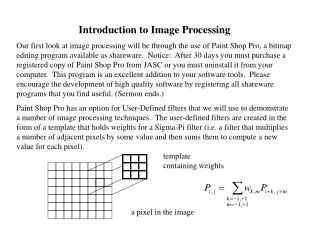
1. Spatial-Frequency Domain: Continuous Fourier Transform Textbook: Chapter 4 (Spatial-Frequency) Blackboard Notes SYDE 575: Introduction to Image Processing

2. Fourier Transform • A signal can be expressed as a weighted sum of sines and cosines Source: Gonzalez and Woods

3. Euler’s Formula • Euler's formula • Based on this, summation of sines and cosines can be expressed as a function of a complex exponential

4. Signal Representation • Any signal f(x,y) can be expressed as a superposition of unit impulses using the sifting property f(x,y) =   f(s,t) d(x-s,y-t) ds dt • Sketch

5. Relationship to Convolution g(x,y) = T[ f(x,y) ] = T [   f( s,t ) d( x - s, y - t ) ds dt ] =   f( s,t ) T[ d( x - s, y - t ) ] ds dt =   f( s,t ) h( x - s, y - t ) ds dt = f(x,y) * h(x,y)

6. Transformation -> Convolution • Transforming a function f(x,y) then involves transforming the impulses which are a function of (x,y) which leads to convolution • Example: 1-D continuous exponential PSF • What is the step response? Edge blur • Can we deblur?

7. Deconvolution • We are able to smooth a signal using an exponential smoothing filter • If we know the blur model, how can we find the original signal f(x,y) for a linear system (where ‘*’ represents convolution): g(x,y) = f(x,y) * h(x,y) • Deconvolution is, in general, not easy to perform

8. Inverse System • As before, to undo the effects of an undesirable affect to the image, generate an inverse system using h(x,y) * h1(x,y) = d(x,y) • Still involves deconvolution! Why is deconvolution difficult? • Each output generally has contribution from many inputs

9. Easier Approach • We prefer to represent f(x,y) with components that are not “smeared” by the LSI (linear, shift invariant) system i.e., {fk,l(x,y) } s.t.Sfk,lfk,l(x,y) = f(x,y) and T [ fk,l(x,y) ] = lk,lfk,l(x,y) so that fk,l(x,y) * h(x,y) = lk,lfk,l(x,y) • Defined as eigenfunctions of LSI systems

10. Complex Exponentials • Complex exponentials, ej2pux, will not be altered by a LTI system • ‘u’ is the frequency of the complex exponential • 1-d: cycles per unit time • 2-d: cycles per unit distance or per degree of visual angle ej2pux * h(x) =  ej2pu(x-s) h(s) ds = [ h(s) e-j2pus ds ] ej2pux = H(u) ej2pux where H(u) represents the continuous Fourier transform (FT) of the function h(x)

11. Continuous Fourier Transform Forward F(u) =  f(x) e-j2pux dx Inverse f(x) =  F(u) e j2pux du • F(u) is complex i.e., F(u) = | F(u) | e jf where | F(u) | is the magnitude and f is the phase

12. Fourier: Magnitude and Phase • Magnitude • Power Spectrum • Phase f(u,v) = tan-1( I(u,v) / R(u,v) )

13. 2D Continuous Fourier Transform Forward F(u,v) =  f(x,y) e-j2p(ux + vy) dx dy Inverse f(x,y) =  F(u,v) e j2p(ux + vy) du dv

14. Important Property • If convolution is performed in the time (1d) or spatial (2d) domain: 1d: g(x) = f(x) * h(x) 2d: g(x,y) = f(x,y) * h(x,y) the transformed functions can be multiplied in the frequency (1d) or spatial frequency (2d) domain: 1d: G(u) = F(u) H(u) 2d: G(u,v) = F(u,v) H(u,v)

15. Examples • Example 1: 1-d local average over window W • Example 2: exponential blur • Example 3: Gaussian blur