Download
1 / 11
110 likes | 213 Views
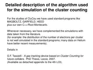
Detailed description of the algorithm used for the simulation of the cluster counting. For the studies of CluCou we have used standard programs like MAGBOLTZ, GARFIELD, HEED plus our own C++/Root Montecarlo. Whenever necessary, we have complemented the simulations with

E N D
Detailed description of the algorithm used for the simulation of the cluster counting For the studies of CluCou we have used standard programs like MAGBOLTZ, GARFIELD, HEED plus our own C++/Root Montecarlo. Whenever necessary, we have complemented the simulations with data taken from the literature. (for example: the distribution of the number of electrons per cluster is not well simulated in the standard programs; many data on Helium have better recent measurements). Details in G.F. Tassielli - A gas tracking device based on Cluster Counting for future colliders. PhD Thesis, Lecce, 2007. (Available as detached appendix to the 4th LOI).
[3] http://www.le.infn.it¥ ∼chiodini¥allow listing¥chipclucou¥tesivarlamava. V. Varlamava. Tesi di Laurea in microelettronica: “Circuito di interfaccia per camera a drift in tecnologia integrata CMOS 0.13 µm”. Universit` a del Salento (2006-2007). [4] http://www.le.infn.it¥ ∼chiodini¥tesi¥Tesi Mino Pierri.pdf. C. Pierri. Tesi di Laurea in microelettronica: “Caratterizzazione di un dis- positivo VLSI Custom per l’acquisizione di segnali veloci da un rivelatore di particelle”. Universit` a del Salento (2007-2008). [1] A. Baschirotto, S. D’Amico, M. De Matteis, F. Grancagnolo, M. Panareo, R. Perrino, G. Chiodini and G.Tassielli. “A CMOS high-speed front-end for cluster counting techniques in ionization detectors”. Proc. of IWASI 2007. A 0.13µm CMOS Front-End for Cluster Counting Technique in Ionization Detectors S. D’Amico1,3, A. Baschirotto2, M. De Matteis1, F. Grancagnolo3, M. Panareo1,3, R. Perrino3, G. Chiodini3, A.Corvaglia3 A CMOS high-speed front-end for cluster counting techniques in ionization detectors A. Baschirotto1, S. D’Amico1, M. De Matteis1, F. Grancagnolo2, M. Panareo1,2, R. Perrino2, G. Chiodini2, G. Tassielli2,3
s tj+1-tj Impact parameter Cluster number
ionizing track drift tube electron . drift distance sense wire impact parameter b ionization clusters ionization act Impact Parameter Resolution mV threshold drift time t1 [0.5 ns units] The impact parameter b is generally defined as: where t1 - t0 is the arrival time of the first (few) e–. b is, with this approach, therefore, systematically overestimated by the quantity: with: ranging from to 1st cluster 2nd cluster
N =12.5/cm r =0.5cm N =12.5/cm r =1cm N =12.5/cm r =2cm N =50/cm r =1cm How large is bmax? Systematic overestimate of b: Usually, though improperly, referred as ionization statistics contribution to the impact parameter resolution
A short note on and Poisson statistics tells us that the number N of ionization acts fluctuates with a variance 2(N) = N. The corresponding variance of = 1/Nis 2() = 1/N42(N) = 1/N3= 3. For a gas with a density of 12.5 clusters/cm and an ionization length of 1 cm, N = 12.5 and = 0.080, with (N) = 3.54 and () = 0.023, or (N)/N = ()/ = 28% Same gas but 2 cm cell gives a factor smaller for both (20%); 0.5 cm cell gives (N)/N = ()/ = 40%. Obviously, in this last case, the error is more asymmetric. COROLLARY 1 For a round (or hexagonal) cell, when the impact parameter grows and approaches the edge of the cell, the length of the chord shortens and the relative fluctuations of N and increase accordingly. COROLLARY 2 Tracks at an angle with respect to the sense wire reduce the error by a factor (sin )-1/2 (e.g. 20% for =45). COROLLARY 3 Sense wires at alternating stereo angles , even at = 0, reduce the error by a factor (cos 2)-1/2 (a few %). In our case, N ionizations are distributed over half chord: 1/(2N) = (/2), and, therefore, (/2) =(/2)3/2= 1/(22)3/2= 1/(22)(). Eventhough < 1> = /4, we’ll assume, conservatively, (1) =(/2)
extreme solutions as defined by the first cluster only “real” track 5 5 5 4 4 4 3 3 3 2 2 2 1 1 sense wire 1 “equi-drift” Can we do any better in He gas mixtures and small cells? First of all, let’s get rid of the systematic overestimate of b by calculating b and 1 from d1 and d2 and assume, for simplicity, that thedi’s are not affected by error(no diffusion, no electronics): from which one gets: and: By generalizing this result with the contribution of the i-th (i2) cluster: the impact parameter can then be calculated by a weighted average with its proper variance: as opposed to:
N = 12.5/cm r = 0.5 cm with <i> b/r with max i 61 m 40 m 28 m Relative gain of (b) as a function of the number of clusters used max i <i> “Real” statistics contribution to (b) From: and its generalization: since
He/iC4H10 = 90/10 (N = 12.5 / cm) r = 1.0 cm Magboltz our exp. points What about diffusion? So far, so good! We have reduced the contribution to theimpact parameter resolutiondue to the ionization statistics at small impact parameter b (where this contribution is dominant since the uncertainty on the drift distance due to electron diffusion is negligible: we have, in fact, assumed so far no error on di’s). What happens as b increases?
(b) with first 2 clusters (b) with first 4 clusters (b) with all clusters 69 m 56 m 49 m Can we do any better? Our previous generalization has brought to the result: b = 0.1 cm b = 0.5 cm b = 0.9 cm
(b) with first 2 clusters (b) with first 4 clusters (b) with all clusters 48 m 41 m 38 m 0 0.5 0.3 0.4 0.2 0.1 Impact parameter resolution with CLUSTER COUNTING first cluster only all clusters in cylindrical drift tubes r = 1.0 cm r = 0.5 cm (N = 12.5 clusters/cm) 145 m 49 m 116 m 38 m