Download
1 / 42
420 likes | 583 Views
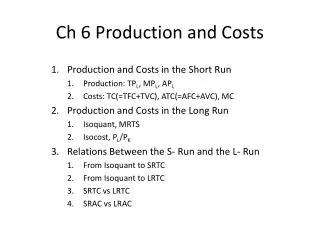
Ch 6 Production and Costs. Production and Costs in the Short Run Production: TP L , MP L , AP L Costs: TC(=TFC+TVC), ATC(=AFC+AVC), MC Production and Costs in the Long Run Isoquant, MRTS Isocost, P L /P K Relations Between the S- Run and the L- Run From Isoquant to SRTC

E N D
Ch 6 Production and Costs Production and Costs in the Short Run Production: TPL, MPL, APL Costs: TC(=TFC+TVC), ATC(=AFC+AVC), MC Production and Costs in the Long Run Isoquant, MRTS Isocost, PL/PK Relations Between the S- Run and the L- Run From Isoquant to SRTC From Isoquant to LRTC SRTC vs LRTC SRAC vs LRAC
1. Basic Short Run Model the output for the production function: Q = 3KL
Swanky Desks Inc.selling handmade desks Production Schedule
Swanky Desks Inc.selling handmade desks Total, Marginal, and Average Products in the Short Run
TP or Q MPL=∆Q/∆L APL=Q/L TPL, MPL, APL Q1 ∆Q ∆L Q1 L L1 L2 L3 L4 L5 L1
APL MPL MPL & APL AP↑ when MP>AP AP↓ when MP<AP MPL APL L L1 L2 L3 L4 L5
When will the APL = MPL? and Why does the APL continue to rise even though the MPL is falling?
Production to Cost L Q Q Q L L
Production Cost Curve (Q#4) Labor 7 6 5 4 3 2 1 1 2.4 4.2 6.4 7.8 8.6 9 TP or Q
Swanky Desks Inc.selling handmade desks Total, Marginal, and Average Products in the Short Run
Swanky Desks Inc.selling handmade desks Cost Schedule (PL=$40 per day & PK=$100 per day)
Swanky Desks Inc.selling handmade desks Cost Schedule (PL=$40 per day & PK=$100 per day)
2. Production and Costs in the Long-runIsoquant Curves • Isoquants: An isoquant demonstrates all the combinations of inputs that produce the same level of output if production is technically efficient. • Not only are isoquants downward sloping, but they bow toward the origin. • slope downward (with more of both inputs, we could always produce more (similar to more-is-better assumption)) • never cross (transitivity and downward slope) • fill the plane (completeness, no matter what combination of inputs used, there will be some level of output) • convex (balanced bundles produce more than bundles with lots of one input and little of the other)
Marginal Rate of Technical Substitution of labor for capital (MRTSLK): the slope of the isoquant if L in on the horizontal axis. • How much capital must be hired to maintain the same level of output if one unit of labor is removed from production. • MRTS: Holding output constant, how capital changes when labor changes by one unit. • MPK: Holding labor constant, how output changes when capital is increased by one unit. • MPL: Holding capital constant, how output changes when labor is increased by one unit. • K*MPK + L*MPL = 0 • K*MPK = -L*MPL • -K/L = MPL/MPK • MRTS = K/L, so MRTS = MPL/MPK
2. Production and Costs in the Long-runIsocost Curves • Isocosts: An isocost curve is a lot like a budget constraint, it reflects all the combinations of inputs that cost the same amount. • PL *L + PK * K = TC
2. Production and Costs in the Long-runCost Minimization • To minimize cost of producing a specific level of Q, we can keep reducing the TC until we can no longer cut cost without producing less than Q’.
2. Production and Costs in the Long-runthe Equimarginal Principle • Start at a point where MRTS < PL/PK. • the benefit of reducing the amount of L used is PL and the cost is MRTS*PK. • Setting the MB = MC results in a level of K and L such that MRTS*PK = PL. • MRTS = PL/PKMPL/MPK=PL/PKMPL/PL=MPK/PK • Expansion Path :As production increases, the locus of tangencies is called the expansion path. It reflects the lowest possible cost of producing any given level of output
2. Production and Costs in the Long-runLong Run Cost Curves • Information needed • Production function or isoquants • Input prices • LRTC: long run total cost – the cost of producing a level of output if production is on the expansion path. • LRAC: long run average cost = LRTC/Q • LRMC: long run marginal cost = LRTC/Q
EXHIBIT 6.11 Deriving Long-Run Total Cost PK=$10 PL=$15 At Q=33, LRTC=? Landsburg, Price Theory and Applications, 7th edition
EXHIBIT 6.12Long-Run Total, Marginal, and Average Costs Landsburg, Price Theory and Applications, 7th edition
Returns to Scale • When all input quantities are increased by 1%, does output go up by • …more than 1% • Increasing returns to scale • Occurs at low levels of output • Long-run average cost curve is decreasing • Caused by either further specialization of resources or technology interacted with size. • …exactly 1% • Constant returns to scale • “What a firm can do one, it can do twice” • Long-run average cost curve is flat • …less than 1% • Decreasing returns to scale • Occurs at sufficiently high levels of output • Long-run average cost curve is increasing • Cuased by bureaucratic intertia. Landsburg, Price Theory and Applications, 7th edition
2. Production and Costs in the Long-runReturns to Scale vs. Economies of Scale. • as Q increases production always exhibits first IRS, then CRS and DRS, • the LRTC looks like this: • the LRAC looks like this:
EXHIBIT 6.13a Short-Run and Long-Run Total Cost Curves Landsburg, Price Theory and Applications, 7th edition
EXHIBIT 6.13b Short-Run and Long-Run Total Cost Curves continued Landsburg, Price Theory and Applications, 7th edition
EXHIBIT 6.15 Many Short-Run Average Cost Curves Landsburg, Price Theory and Applications, 7th edition
3. Relationship between the SR and LR PK=200, PL=20 TC1 =8000+5500=13,500 TC2SR=8000+6420=14,420 TC2LR=8400+5740=14,140
3. Relationship between the SR and LRis LRMC higher or lower than MC? SRTCK=40 14,420 14,140 13,500 8400 8000 SRTCK=42 135 140 MC is 920/5 = 184 LRMC = 640/5 = 128
3. Relationship between the SR and LRis LRMC higher or lower than MC? MC is 920/5 = 184 LRMC = 640/5 = 128
3. Relationship between the SR and LRis LRMC higher or lower than MC?
3. Relationship between the SR and LRis LRMC higher or lower than MC?