Download

1 / 20
210 likes | 284 Views
This study applies a semi-distributed version of the SAC-SMA hydrologic model to simulate streamflow in the Illinois River Basin. The model uses data such as DEM, hourly streamflow, precipitation, and more to calibrate and evaluate simulations at the basin outlet and interior points. Spatial resolution criteria for sub-basin delineation and calibration scenarios are discussed, highlighting the effectiveness of the Semi-Lumped parameter scenario in this homogeneous basin. The study also explores potential improvements in streamflow simulations and ongoing research on PE adjustment factors and channel cross-sections. It concludes that the calibrated model leads to improved simulation results compared to uncalibrated simulations, demonstrating the potential of the SAC-SMA model in enhancing streamflow predictions.

E N D
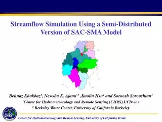
Behnaz Khakbaz1, Newsha K. Ajami 2 ,Kuolin Hsu1 and Soroosh Sorooshian1 1Center for Hydrometeorology and Remote Sensing (CHRS),UCIrvine 2 Berkeley Water Center, University of California,Berkeley Streamflow Simulation Using a Semi-Distributed Version of SAC-SMA Model
Study River Basin : Illinois River Basin South of Siloam Spring, AR • Basin Area : 1489 km2 General View • Model: A Semi-Distributed Version of SAC-SMA • Data used in the study: • 30m resolution DEM • Basin boundary • Hourly streamflow data (USGS) • Vegetation • Inputs to the model: • Multisensor (NEXRAD +Gauge) precipitation data • Mean Free Water Surface Evaporation Data • Interested in: • Calibrated and uncalibrated simulations at • -The outlet of the basin • -The interior points
Spatial and Temporal Resolution The criteria for sub-basin delineation: considering the confluents the specified interior points 15 Sub-basins Area of Sub-basins : 5 – 200km2 Average area : 100km2 Temporal Resolution: 1hr
Extracting MAP from Multi-Sensor(NEXRAD+Gauge) Precipitation Data
Hydrologic Model SACramento Soil Moisture Accounting model (SAC-SMA) • Used in NWS • Deterministic • Lumped • Non-linear
Our Model Structure Overland flow Routing Sub-basin Outlet Bypass overland flow routing KW Routing along channel n = 0.025,Wb=35m (Ajami et al,2004)
Lc L Derivation of UH for Sub-basins Empirical formulas tl = Ct ( L*Lc)0.3 tp = D/2 + tl Qp = 0.208 * A / tp Ct =0.6/S0.5 tl: lag time(hr) D:effective rainfall duration(hr) A: basin area(km2) tp:time to peak(hr) Qp:peak discharge(cms) Outlet
Sub-basin Outlet KW Routing along the channel Model Parameters Parameters to be calibrated No parameter from overland flow and channel routing to be calibrated
f fi ,i=1,..,15 f1=...=f15 fi ,i=1,..,15 f1=...=f15 Calibration Scenarios Semi-Lumped (SL): Distributed Input Lumped Parameters Semi-Distributed (SD): Distributed Input Distributed Parameters Lumped (L): Lumped Input Lumped Parameters
Semi-distributed Calibration Scenario Using SAC-SMA parameter grids (Koren et al, 2000) for 11 parameters as apriori information in semi-distributed calibration scenario Pij=APij /APbj*Pj Pij: Adjusted Parameter j for sub-basin i APij: Averaged a priori parameter j for sub-basin i APbj: Averaged a priori parameter j for whole basin Pj : Common parameter j for all the sub-basins i=1,2,…,15 sub-basin j=1,2,…,11 parameter only 13 parameters(as opposed to 13*15=195) to be calibrated Similar to Vieux et al (2004) and Frances et al(2007)
Places strong weights on low flow parts:Having good estimate of LZ params Places strong weights on high flow parts:Having good estimate of UZ params Calibrating LZ params To re-adjust them Calibration Tool and Method Calibration Tool:Shuffled Complex Evolution (SCE-UA)(Duan et al,1992) Multi-Step Automatic Calibration Scheme (Hogue et al , 2000)
Sandy Loam Silty Loam Loam Uncalibrated:A Priori Parameters Zup=5.08(1000/CN-10)/(Ts-Tfld)
Statistical Results of Simulations for the Outlet in Calibration Period
Conclusion Uncalibrated simulations using a priori SAC-SMA parameters (Koren et al,2000) in the semi-distributed SAC-SMA are reasonably good. Calibration of the model can improve the simulation results comparing to the uncalibrated simulations. • Comparison of different calibration scenarios tried in our model shows • the best performance for Semi-Lumped parameter scenario for the outlet .This • result is somehow expected for a relatively homogeneous basin like Illinois • river basin at Siloam Spring. • Semi-distributed version of SAC-SMA has the potential toimprove the streamflow simulations at the outlet and meanwhile provide streamflow simulations for specified interior points .
On-going Study • Potential Evapotranspiration: PE adjustmentfactors • using Global Vegetation Fraction (GVF) • Roughness Coefficients • Channel Cross Sections
4-90.4% 8-3.3% 12-2.2% 13-2.1% 14-2% Vegetation
PET PEadj factors: Using Multi-year averaged Global Vegetation Fraction (GVF) for 52 weeks of a year and the relationship between GVF and PEadj factors(Koren et al 1998,unpublished report) GVF dataset derived from 25 years AVHRR data and extracted from the NOAA/NESDIS website
Roughness Coefficients There were no cross-sections and roughness coef available for Illinois River basin above Siloam Spring. Empirical equation derived by Tokar and Johnson 1995, cited by Koren et al, 2003: nc= no Sc0.272 F-0.00011 F: upstream drainage area , Sc: slope of each channel section no estimated from the measurements at the basin outlet : USGS flow measurements at the basin outlet
Channel Cross Sections Leopold & Madock (1953) cited in Frances et al(2007): Wb=a1 Qba1 Wb=a1 (k Af)a1 Qb= k Af Wb=Wo Af.a1 Wb : top width , Qb:bankfull discharge , A: drainage area to a particular section Frances et al(2007): f=0.75, a1=0.5 Assuming rectangular cross-sections and using the basin outlet data to estimate Wo