Subgraph Search Over Large Graph Database

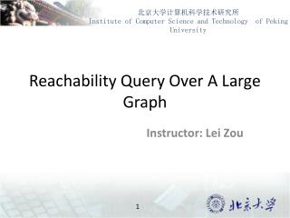
1. 北京大学计算机科学技术研究所 Institute of Computer Science and Technology of Peking University Subgraph Search Over Large Graph Database Instructor: Lei Zou

2. Outline • Subgraph Isomorphism Algorihtm Ullmann Algorithm; VF2 Algorithm QuickSI • Subgraph Search Over a large collection of graphs GraphGrep, gIndex, Closure-Tree, Gcode • Subgraph Search Over a Single Large Graph

3. Problem Definition Given a graph database and a query graph, discover all graphs containing this query graph. Sample database query graph (a) (b) (c) Query graph

4. Applications • Chemical Informatics (chemical compound) • Bioinformatics (protein structure, pathway) • Workflow • XML • … Graph Database Management

5. Scalability Issue • Sequential scan is not scalable • Disk I/O • Subgraph isomorphism testing • An indexing mechanism is needed • DayLight: Daylight.com (commercial) • GraphGrep: Dennis Shasha etc. PODS'02 • Grace: Srinath Srinivasa etc. ICDE'03

6. GraphGrep (shasha et al. PODS02) • Fingerprinting: to filter the database • A subgraph matching algorithm

7. Concept Use small components of the query graph and of the database graphs to filter the database and to do the matching

8. Graph == Sets of “Paths” 0 3 C B lp = 4 A={(1)} AB={(1, 0), (1,2)} AC ={(1, 3)} ABC={(1,0,3), (1,2,3)} ACB={(1, 3, 0), (1,3,2)} ABCA={(1 ,0 ,3 ,1),(1, 2, 3, 1)} ABCB ={(1 ,2,3 ,0),(1, 0, 3, 2)} B={(0),(2)} BA={(0,1),(2,1)} BC={(0,3), (2, 3)} ….……. B 1 2 A 1 A 1 A 1 A 1 A lp = 2 0 2 B B 3 3 C C C C lp = 3 B B 3 3 0 2 lp = 4 2 B 0 B 1 A 1 A

9. Fingerprint D 1 0 B 0 3 C B C B 2 3 C 4 B C E B 1 2 A 1 2 3 A B A 4 5 6 Graph g3 Graph g2 Graph g1

10. Patterns in a Query lp = 4 A*BCA*CB 1 A C 2 B 0 B 3 2 3 C 0 A B B lp= 3 A* BC, CB CA* 1

11. Filter the Database 0 3 C B 0 B 2 1 A C 4 B B C A 1 2 3 Graph g1 1 Discarded Graph g3 C D 1 B 0 B C 2 3 2 3 E B A B A 4 5 6 Query Discarded Graph g2

12. 1 C B 0 2 3 A B Subgraph Matching 0 3 C B A*BCA* CB 2 1 A B Graph g1 Query ABCA = {(1, 0, 3, 1),(1, 2, 3, 1)} CB = {(3,0),(3,2)} Select the set of paths in g1 matching the patterns of the query ABCACB = {((1, 0, 3, 1),(3, 0)), ((1, 0, 3, 1),(3, 2)),((1, 2, 3, 1),(3, 0)), ((1, 2, 3, 1),(3, 2))} Combine any list from ABCA with any list of CB accordingly ‘*’ and ‘_’ ABCACB ={removed, ((1, 0, 3, 1),(3, 2)),((1, 2, 3, 1),(3, 0)), removed} Remove lists if they contains equal nodes in the positions not involved above

13. gIndex (Yan et al. @SIGMOD 04) Query graph (Q) Graph (G) If graph G contains query graph Q, G should contain any substructure of Q Substructure Remarks • Index substructures of a query graph to prune graphs that do not contain these substructures

14. Framework • Two steps in processing graph queries Step 1. Index Construction • Enumerate structuresin the graph database, build an inverted index between structures and graphs Step 2. Query Processing • Enumerate structuresin the query graph • Calculate the candidate graphs containing these structures • Prune the false positive answers by performing subgraph isomorphism test

15. Cost Analysis Query Response Time Disk I/O time Isomorphism testing time Query indexing time Size of candidate answer set Remark: make |Cq| as small as possible

16. Path-Based Approach Sample database (a) (b) (c) Paths 0-length: C, O, N, S 1-length: C-C, C-O, C-N, C-S, N-N, S-O 2-length: C-C-C, C-O-C, C-N-C, ... 3-length: ... Built an inverted index between paths and graphs

17. Path-Based Approach (cont.) Query graph 0-length: SC={a, b, c}, SN={a, b, c} 1-length: SC-C={a, b, c}, SC-N={a, b, c} 2-length: SC-N-C = {a, b}, … … Intersect these sets, we obtain the candidate answers - graph (a) and graph (b) - which may contain this query graph.

18. Problems of Path-Based Approach Sample database (a) (b) (c) Query graph Graph (c) contains this query graph. However, if we only index paths: C, C-C, C-C-C, C-C-C-C, we can not prune graph (a) and (b).

19. Disadvantages of Path-Based Approach • Paths are simple, structural information is lost • There are too many paths We propose • Use structures instead of paths • Use discriminative structures

20. gIndex: Indexing Graphs by Data Mining • Identify frequent structures in the database, the frequent structures are subgraphs that appear quite often in the graph database • Prune redundant frequent structures to maintain a small set of discriminative structures • Create an inverted index between discriminative frequent structures and graphs in the database

21. Frequent Structures Sample database (a) (b) (c) Frequent structures with support 2 (a) (b)

22. Frequent Structures (cont.) • Efficient frequent graph mining algorithms are available Apriori: • AGM/AcGM: Inokuchi et al (PKDD’00) • FSG, Kuramochi et al (ICDM’01) • Vanetik et al (ICDM’02) Pattern-growth: • MoFa, Borgelt et al (ICDM’02) • gSpan: Yan and Han (ICDM’02) • …

23. Frequent Structures: Threshold Issue • How to set up the minimum support threshold? • If it is too low, it may generate too many frequent graphs • If it is too high, it may miss important structures • Should we enforce a uniform threshold for the different size of structures? Size-increasing support threshold

24. Frequent Structures: Threshold Issue • Intuition: large structures with low support will likely be indexed well by their substructures that have the similar support • Size-increasing support threshold • The support threshold increases when the indexed structures become larger

25. Frequent Structures: Volume Issue • The number of frequent structures may exceed the number of graphs in the database when the support is low • 1,000 graphs may generate 1,000,000 frequent structures • It is time and memory expensive to compute and index all frequent structures discriminative structures

26. Redundant Structures Sample database • All graphs contain structures: C, C-C, C-C-C • Why bother indexing these redundant frequent structures? • Remove these redundant structures • Only index structures that provide more information than existing structures (a) (b) (c)

27. Discriminative Structures

28. Discriminative Structures • Pinpoint the most useful frequent structures • Given a set of sturctures and a new structure , we measure the extra indexing power provided by , When is small enough, is a discriminative structure and should be included in the index • Index discriminative frequent structures only • Reduce the index size by an order of magnitude • Achieve good performance

29. Discriminative Structures

30. GIndex - Construction • First generates all frequent fragments while taking out redundant ones • Translates fragments into sequences and holds them in a prefix tree • Each fragment has an id list: the ids of the graphs containing the fragment • Graph Sequentialization (DFS Code) • Labeled edge is a 5-tuple (I,j,li, l(I,j),lj) • Described in another paper

31. GIndex - Construction • gIndex Tree • each fragment can be mapped to an edge sequence (DFS code), insert the edge sequences of discriminative fragments in a prefix tree called the gIndex Tree

32. GIndex - Search

33. GIndex - Search • Optimization • Apriori Pruning • If a fragment is not in the gIndex tree, we need not check its super-graphs

34. GIndex - Search • Verification • After getting the candidate answer set, we have to verify that the graphs in the set really contain the query graph • perform a subgraph isomorphism test on each graph one by one

35. Graph Query Processing • Chemical Compounds (a) caffeine (b) diurobromine (c) viagra • Query Graph

36. Precise vs. Approximate Search in Graphs • Given a graph database and a query graph Q, • Find graphs containing Q exactly • (Precise Matching, gIndex, SIGMOD’04) • Find graphs containing Q approximately (Approximate Matching, Grafil)

37. Evaluating Graph Similarity 1. Maximal Common Subgraph (MCS): Given two graphs Q and G, assume that S is subgraph isomorphism to both Q and G. S is called a common subgraph of Q and G. The MCS between Q and G is the common subgraph with the largest number of edges (|E(S)|).

38. Evaluating Graph Similarity MCS A E B C A B F C Q G

39. Evaluating Graph Similarity 2. Minimal Graph Edit Distance The minimal edit distance between Q and G is the minimal number of edit operations (insertion, deletion, or relabeling ) in the optimal alignments that make Q reach G.

40. Evaluating Graph Similarity 2. Minimal Graph Edit Distance A E B C B C F A Q G

41. Solution (I) • Compute the similarity between the graphs in the database and the query graph directly (costly) • sequential scan • subgraph similarity computation

42. Solution (II) • Form a set of subgraph queries from the original query graph and use the exact subgraph search (costly) • If we allow 3 edges to be missed in a 20-edge query graph, it may generate 1,140 subgraphs.

43. Scalability Issue • Sequential scan is not scalable • Disk I/O • Approximate subgraph isomorphism testing • It takes minutes to finish a graph query • A strategy of indexing and searching is needed Prune candidates as many as possible

44. Index Needed ! • Precise Search • Use frequent patterns as indexing features • Select features in the database space based on their selectivity • Build the index • Approximate Search • Hard to build indices covering similar subgraphs – explosive number of subgraphs in databases • Idea: (1) keep the index structure (2) select features in the query space

45. Substructure Similarity Measure • Structure-based similarity measure • The largest overlapping part of two graphs • Relaxation: the number of edges that can be relabeled or deleted (relaxation of the query graph) G Q

46. Structural Features Graph Database (a) (b) (c) Structural Features (small fragments) • atom • path • bond • subgraph

47. Substructure Similarity Measure • Feature-based similarity measure • Each graph is represented as a feature vector X = {x1, x2, …, xn} • The similarity is defined by the distance of their corresponding vectors • Easy to index • Very fast • Rough measure

48. Substructure Similarity Search • Structure-based similarity • Accurate measure • Slow Can we transform structure-based to feature-based? • Feature-based similarity • Rough measure • Fast

49. Intuition Graph (G1) • If graph G contains the major part of a query graph Q, G should share a number of common features with Q Query (Q) Graph (G2) • Given a relaxation ratio, calculate the maximal number of features that can be missed ! Substructure At least one of them should be contained

50. Feature-Graph Matrix • An occurrence table between feature and graph Assume a query graph has 4 features and only 1 feature to miss due to the relaxation threshold