Download
1 / 37
370 likes | 520 Views
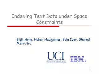
Indexing Text Data under Space Constraints. Bijit Hore , Hakan Hacigumus, Bala Iyer, Sharad Mehrotra. Introduction. We want to design an efficient indexing technique to support pattern matching queries over string data We focus on LIKE queries in SQL :

E N D
Indexing Text Data under Space Constraints Bijit Hore, Hakan Hacigumus, Bala Iyer, Sharad Mehrotra
Introduction We want to design an efficient indexing technique to support pattern matching queries over string data We focus on LIKE queries in SQL: • Select * from R where R.A Like “dat_”; • Select * from R where R.A Like “d%”; Contribution: Aq-grambased index for efficient pattern matching q-gram: any string of symbols of length q,from ∑
The basic approach Given (initially): Q: A typical workload of query patterns R: The set of record strings to be indexed Generic approach to evaluate LIKE queries: • Generate a set of candidate grams G • Select an “appropriate” set I ⊆ G • Create an index using I where : where every g I has a pointer to r R iff r ∋ g • Given a query q, get all g q from I and return the intersection of their pointer lists • Discard the false positives from the returned list
Research Issues • Generating an appropriate set of candidate grams G relevant to workload Q • Choosing an optimal index set I ⊆ G minimizes the # false positives over Q 3. Data structures / Query processing methodology *
Outline • Introduction • Optimal Gram Selection • Complexity and optimizations • A parallel algorithm for gram selection • Workload reduction • Experiments & Conclusion
Visualizing the Q-G-R relations R G Q r1 q1 _an% San Jose r2 Los Angeles, International r3 q2 %York% g1 John F Kennedy, New York an r4 g2 La Guardia, New York q3 San Franc% or r5 Newark g3 r6 ne San Francisco q4 %kane% r7 Benefit(g) = (# queries ∋ g) X (# records ∌ g) Oakland Gram “ne” covers the pairs {(q4,r1), (q4,r2), (q4,r6), (q4,r7)}
Optimal gram selection for index Given: • 3 setsQ, G, R(workload, candidates, records) • Weight functionweight(q): Q ℜ • Cost functioncost(g):G ℜ • Budget constraintM • Define a map:cover(g) : G Q X R set of all(q,r)pairs s.tq ∋ g& r ∌g (weight(q,r) = weight(q)) Formal definition: BestIndex(Q,R,G,M) = Imax⊆ G, where weight(Imax) is maximized over all I ⊆ G & cost(Imax) ≤ M
Benefit of a gram Benefit(g) = (# queries ∋ g) X (# records ∌ g) A greedy heuristic for top-k grams that does not work: Include the k grams with the largest individual benefits in I Cause: A gram g* might have high individual benefit BUT In presence of other grams in I, g* might not prune any new records for any of the queries ∋ g*
NP-hardness & an approximation algorithm BestIndex problem is NP-Hard (reduction from set cover) Define: benefit(g,I) = total weight of new (q,r) pairs covered by g (not already covered by some gram I) utility(g,I)= Heuristic: In every iteration add the gram with the highest utility, till cost budget is exhausted The greedy heuristic gives a 0.5(1-)optimal approximation [2]
BestIndex algorithm: Example Example: choose top 2 grams for the G-(Q,R) matrix shown below : (q,r) G • First iteration: compute utility of all candidates • cost(g1) = 3; cost(g2) = 2; cost(g3) = 3 • utility(g1) = 9/3 = 3; utility(g2) = 5/2 = 2.5; utility(g3) = 8/3 = 2.66 • Top gram is g1 (utility(g1) > utility(g3) > utility(g2)) • Second iteration: • utilities change: utility(g2) = 5/2 > utility(g3) = 3/3 choose g2
Compact representation of G-(Q,R) relations (q,r) G 1 1 0 S R Q G G S[g][(q,r)] = (~M1[g][r]) & M2[g][q] M1 M2
Complexity of an iteration (q,r) G Complexity of single iteration Ο(|Q|*|R|*|G|) !
Outline • Introduction • Optimal Gram Selection • Complexity and optimizations • A parallel algorithm for gram selection • Workload reduction • Experiments & Conclusion
Complexity of the naïve algorithm • Time complexity (worst case) = O(|I|*|R|*|Q|*|G|) for choosing an set I of indexing grams • Space complexity = O( |G|*|Q| + |G|*|R| )…matrices M1 and M2 • The naïve algorithm scales poorly with problem size • Explore the following optimization approaches: • Pre-processing: pruning, auxiliary data structures • Parallelization • Workload compression
Parallelizing the BestIndex algorithm R G Q r1 q1 r2 r3 q2 g1 r4 g2 q3 r5 g3 r6 q4 r7
Parallelizing the BestIndex algorithm R G Q r3 r3 q2 r4 g2
Parallelizing the BestIndex algorithm R G Q r1 r2 g1 q3 r6 r7
Parallelizing the BestIndex algorithm R G Q r1 r2 Complexity of each gram-selection iteration reduces from O(|Q|*|R|*|G|) to O(|Q|*|R|) r3 g1 r4 r5 g3 r6 q4 r7
Outline • Introduction • Optimal Gram Selection • Complexity and optimizations • A parallel algorithm for gram selection • Workload reduction • Experiments & Conclusion
Workload reduction Parallel algorithm complexity: O(|I|*|Q|*|R|)(worst case) Explore ways of reducing the workload Q while trying to minimize loss of quality (similar to [4]) Our approach: • Define appropriate distance measures between queries • Use k-median clustering to form k query clusters • Fold all queries in a cluster onto the median query • These k medians form the compressed workload Q’
Family of MaxDevDist measures • MaxDevDist(q1,q2) assumes q1 is folded onto q2 • Folding affects benefits of grams in: (G1-G2) ∪ (G2–G1) Gi is the set of grams in qi • Variants proposed, proportional to: • |R’((G1-G2) ∪ (G2–G1)) | • 1 / |R’(G2 )| • 1 / |R’(G1∩ G2 )| • R’(g) = set of records not containing g
Candidate set generation Generate candidate set of gramsG using Q: • Build a suffix tree by inserting suffixes of all q ∈ Q • Set of all path-labels G0 • Retain shortest, mutually distinguishable prefixes of the path-labels in G0 with selectivity < sthresh G r an e$ Franc$ n ork$ kane$ York$ $ e$ c$ $ e$ k$ anc$ Suffix tree on Q = { _an%, %York%, %Franc%, %kane } G0 = { an, anc, ane, e, Franc, kane, n, ne, ork, r, rk, ranc, York }
Outline • Introduction • Optimal Gram Selection • Complexity and optimizations • A parallel algorithm for gram selection • Workload reduction • Experiments & Conclusion
Experimental results Data Sets: The “Digital Bibliography & Library Project “ 2 string attributes: <author, publication> • |R| ≈ 305,000 records • |Q| = 1000, 2000, 3000 & 4000 (author last-names) • |G| ≈ 4K, 9K, 12K, 15K for the respective query sets Performance metric: Average Relative Error (ARE):
Performance • Plots compare the performance of our index with that of FREE [1] (we plot the average relative error) • FREE does not consider any query model unlike BestIndex • FREE generates all grams up to a certain length and uses a cut-off selectivity for discarding candidates
Resilience to deviation from workload • We test the resilience of our index by deviating the test query set from the workload that is used to build it
Workload Reduction • MaxDevDist_2 performs the best • Random sample is worst !
Conclusions • We show that“Optimal gram selection for indexing in presence of workload & storage constraint”, is NP-hard • Adapt a0.5(1- )approximation algorithm to select grams optimally BestIndex • Speedup through Parallelizationof code • Exploreworkload reductiontechniques • Experimental result comparing with previous approaches BestIndex is superior !
References • Cho, J., Rajagopalan, S., “A Fast Regular Indexing Engine” ICDE 2002 • Khuller, S., Moss, A., Naor, J., “The Budgeted Maximum Coverage Problem”, IPL, V-70 • Ukkonen, E., “Online construction of suffix trees”, Algorithmica • Chaudhury, S., Gupta, A., K., Narasayya. V, “Compressing SQL Workloads”, ACM SIGMOD ‘02
BestIndex algorithm BestIndex-Naive(Q,R,G,M) • while some (q, r) uncovered AND space available • for every gram g ∈ G \ I set benefit[g] = 0 • for everyuncovered (qk,rj) • for everycandidate gi not in I • if(gi covers (qk, rj)) then • benefit[gi] = benefit[gi] + 1 • if (∃ a g with benefit[g] > 0) then • for every candidate g • utility[g] = benefit[g] /cost(g) • else EXIT • I = I ∪ {gmax}, where gmaxhas maximum utility • end Ο(|Q|*|R|*|G|)
Pre-processing optimizations Pruning: Discard frequent grams from G (we pruned all grams with selectivity ≥ 0.1) Auxiliary data structure: Observation: To compute the benefit of a gram for a query qk : • Need only grams contained in qk G(qk) • Need only the set of records spanned by G(qk) To allow such selective access for benefit computation, create 2 lists : Q-G-list andG-R-list
The auxiliary data structures Q-G-list G-R-list q1 g1 G(qk) q2 g2 R(gi) q3 g3 Size is a small G-R-list helps in parallelizing the problem q|Q| Q-G-list reduces the complexity of each gram-selection iteration from O(|Q|*|R|*|G|) to O(|Q|*|R|) g|G|
Parallel BestIndex algorithm Parallelizable BestIndex(Q,R,G,M) • Partition the original problem : P1 … P|Q| • While (budget not filled & all (q,r) not covered) • For all g ∈G \ I benefitglobal(g) 0 • For each sub-problem Pi • Compute local benefits g ∈Gi: benefiti(g) • benefitglobal(g) benefitglobal(g) +benefiti(g) • I I ∪ {g*} where g* has highest global utility • Return I The time complexity O (|I|*(|R1|+…+|R|Q||)) = O (|I|*|Q|*Avg(|Ri|)) For our data Avg(|Ri|) ≈ 0.17|R| ≈ 6 times faster than naïve + basic optimized code, even for sequential execution)
Distance measures Maximum Deviation Distance measures (MaxDevDist) • Let Ibest BestIndex(Q) & I’ BestIndex(Q’) • MaxDevDist tries to capture the notion of “how different is I’ from Ibest” • Intuition: • Difference in Ibest & I’ depends on benefit(g) computed for candidate grams in each case • benefit(g) α |R’(g)| where R’(g) = set of records not containing g
Distance measure (example) Q = {q1 , q2} = {ab , bb} G1 = {a, b, ab}; G2 = {b, bb} G1 – G2 = {a, ab}; G2 – G1 = {bb}; G1∩ G2= {b} (G1 – G2) ∪ (G2 – G1) = {a, ab, bb} Let |R| = 10, |R(a)| = 7 |R’(a)| = 3 |R(a)| = 5 |R’(a)| = 5 |R(a)| = 2 |R’(a)| = 8 |R(a)| = 1 |R’(a)| = 9 MaxDevDist1(q1, q2) = =
A measure of quality of Index Quality of index I w.r.t workload Q can be measured by: Aggregate Proportion of Error (APE) APE (Q,I) =