CASE STUDY : Genetic Linkage Analysis via Bayesian Networks

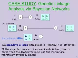
1. D A2/A2 H A1/A1 1 2 H A2/A2 H A1/A2 3 4 H | D A2 | A2 H D A1 A2 D D A2 A2 D D A1 A2 Recombinant D A1/A2 5 CASE STUDY: Genetic Linkage Analysis via Bayesian Networks Phase inferred We speculate a locus with alleles H (Healthy) / D (affected) If the expected number of recombinants is low (close to zero), then the speculated locus and the marker are tentatively physically closed.

2. The Variables Involved Lijm = Maternal allele at locus i of person j. The values of this variables are the possible alleles li at locus i. Lijf = Paternal allele at locus i of person j. The values of this variables are the possible alleles li at locus i (Same as for Lijm) . Xij= Unordered allele pair at locus i of person j. The values are pairs of ith-locus alleles (li,l’i). “The genotype” Yj= person I is affected/not affected. “The phenotype”. Sijm= a binary variable {0,1} that determines which maternal allele is received from the mother. Similarly, Sijf= a binary variable {0,1} that determines which paternal allele is received from the father. It remains to specify the joint distribution that governs these variables. Bayesian networks turn to be a perfect choice.

3. Si3f Li2f y2 Xi2 Li2m Li3f Xi3 Li3m Y3 Li1f Xi1 Y1 Li1m Si3m Locus 2 (Disease) Locus 3 Locus 4 Locus 1 The Bayesian network for Linkage This network depicts the qualitative relations between the variables. We have already specified the local conditional probability tables.

4. L11m L11f L12m L12f X11 S13m X12 S13f L13f L13m X13 Details regarding recombination L21m L21f L22m L22f X21 S23m X22 S23f Y2 Y1 L23f L23m X23 Y3  is the recombination fraction between loci 2 & 1.

5. Li1f Li1m Xi1 Si3m Y1 Li3m Details regarding the Loci P(L11m=a) is the frequency of allele a. X11 is an unordered allele pair at locus 1 of person 1 = “the data”. P(x11 | l11m, l11f) = 0 or 1 depending on consistency The phenotype variables Yj are 0 or 1 (e.g, affected or not affected) are connected to the Xij variables (only in the disease locus). For example, model of perfect recessive disease yields the penetrance probabilities: P(y11 = sick | X11= (a,a)) = 1 P(y11 = sick | X11= (A,a)) = 0 P(y11 = sick | X11= (A,A)) = 0

6. SUPERLINK • Stage 1: each pedigree is translated into a Bayesian network.  • Stage 2: value elimination is performed on each pedigree (i.e., some of the impossible values of the variables of the network are eliminated). • Stage 3: an elimination order for the variables is determined, according to some heuristic. • Stage 4: the likelihood of the pedigrees given the  values is calculated using variable elimination according to the elimination order determined in stage 3. • Allele recoding and special matrix multiplication is used.

7. X1 X1 X2 X2 X3 X3 Xi-1 Xi-1 Xi Xi Xi+1 Xi+1 Comparing to the HMM model S1 S2 S3 Si-1 Si Si+1 X1 X2 X3 Yi-1 Xi Xi+1 The compounded variable Si = (Si,1,m,…,Si,2n,f)is called the inheritance vector. It has 22n states where n is the number of persons that have parents in the pedigree (non-founders). The compounded variable Xi = (Xi,1,m,…,Xi,2n,f) is the data regarding locus i. Similarly for the disease locus we use Yi. REMARK: The HMM approach is equivalent to the Bayesian network approach provided we sum variables locus-after-locus say from left to right.

8. over 100 hours Out-of-memory Pedigree size Too big for Genehunter. Experiment A (V1.0) Elimination Order: General Person-by-Person Locus-by-Locus (HMM) • Same topology (57 people, no loops) • Increasing number of loci (each one with 4-5 alleles) • Run time is in seconds.

9. Software Order type Bus error Out-of-memory Experiment C (V1.0) • Same topology (5 people, no loops) • Increasing number of loci (each one with 3-6 alleles) • Run time is in seconds.

10. Some options for improving efficiency • Multiplying special probability tables efficiently. • Grouping alleles together and removing inconsistent alleles. • Optimizing the elimination order of variables in a Bayesian network. • Performing approximate calculations of the likelihood.

11. Standard usage of linkage There are usually 5-15 markers. 20-30% of the persons in large pedigrees are genotyped (namely, their xij is measured). For each genotyped person about 90% of the loci are measured correctly. Recombination fraction between every two loci is known from previous studies (available genetic maps). The user adds a locus called the “disease locus” and places it between two markers i and i+1. The recombination fraction ’between the disease locus and marker i and ” between the disease locus and marker i+1 are the unknown parameters being estimated using the likelihood function. This computation is done for every gap between the given markers on the map. The MLE hints on the whereabouts of a single gene causing the disease (if a single one exists).

12. Relation to Treewidth • The unconstrained Elimination Problem reduces to finding treewidth if: • the weight of each vertex is constant, • the cost function is • Finding the treewidth of a graph is known to be NP-complete (Arnborg et al., 1987). • When no edges are added, the elimination sequence is perfect and the graph is chordal.

13. Parameter Estimation Lecture #10 Acknowledgement: Some slides of this lecture are due to Nir Friedman. .

14. Where  ={1,2,3,4,5} are called the parameters of the likelihood function. We wish to estimate these parameters from the data we have seen. Likelihood function for a die: Multinomial sampling Let X be a random variable with 6 values x1,…,x6 denoting the six outcomes of a die. Suppose we observe a sequence of independent outcomes: Data = (x6,x1,x1,x3,x2,x2,x3,x4,x5,x2,x6) What is the probability of this data ? If we knew the long-run frequencies i for falling on side xi, then,

15. Sufficient Statistics • To compute the probability of data in the die example we only require to record the number of times Ni falling on side i (namely,N1, N2,…,N6). • We do not need to recall the entire sequence of outcomes • {Ni | i=1…6} is called the sufficient statistics for the multinomial sampling.

16. Datasets Statistics Sufficient Statistics • A sufficient statistics is a function of the data that summarizes the relevant information for the likelihood • Formally, s(Data) is a sufficient statistics if for any two datasets D and D’ • s(Data) = s(Data’ ) P(Data|) = P(Data’|)

17. A sufficient condition for maximum is: Maximum Likelihood Estimate Maximum likelihood estimate is an assignment to the parameters that maximizes the probability of data (i.e., the likelihood function ). Usually one maximizes the log-likelihood function which is easier to do and gives an identical answer:

18. We have just found that: Divide the ith and jth equations: Sum from j=1 to 6: Hence the MLE is given by: Finding the Maximum

19. The MAP estimate is given by The six pseudo counts N’i sum to N’. They express one’s assessment regarding the frequencies for each side prior to seeing the data. Large N’ indicates high confidence. Smaller than 1 values are possible. The MAP estimate can be justified as maximizing one’s posterior (namely, after seeing the data) best estimate of the frequencies for each side. The theory formally justifying this formula is called Bayesian Statistics (not covered in this course due to time constraints). Adding Pseudo Counts The MLE given by can be misleading for small data sets because it could happen that a small data set is not typical. For example, it might be that we know that the dice is manufactured to be loaded but the small dataset we examined does not show this property.

20. The ABO locus has six possible genotypes {a/a, a/o, b/o, b/b, a/b, o/o}. The first two genotypes determine blood type A, the next two determine blood type B, then blood type AB, and finally blood type O. We wish to estimate the proportion in a population of the 6 genotypes. Suppose we randomly sampled N individuals and found that Na/a have genotype a/a, Na/b have genotype a/b, etc. Then, the MLE is given by: Example: The ABO locus Recall that a locus is a particular place on the chromosome. Each locus’ state (called genotype) consists of two alleles – one parental and one maternal. Some loci (plural of locus) determine distinguished features. The ABO locus, for example, determines blood type.

21. The ABO locus (Cont.) However, testing individuals for their genotype is a very expensive test. Can we estimate the proportions of genotype using the common cheap blood test with outcome being one of the four blood types (A, B, AB, O) ? The problem is that among individuals measured to have blood type A, we don’t know how many have genotype a/a and how many have genotype a/o. So what can we do ? We use the Hardy-Weinberg equilibrium rule that tells us that in equilibrium the frequencies of the three alleles a,b,o in the population determine the frequencies of the genotypes as follows: a/b= 2a b, a/o= 2a o, b/o= 2b o, a/a= [a]2, b/b= [b]2, o/o= [o]2. So now we have three parameters that we need to estimate.

22. What is the probability of Data={B,A,B,B,O,A,B,A,O,B, AB} ? Obtaining the maximum of this function yields the MLE. This can be done by multidimensional Newton’s algorithm. The Likelihood Function Let X be a random variable with 6 values xa/a, xa/o ,xb/b, xb/o, xa/b , xo/o denoting the six genotypes. The parameters are = {a ,b, o}. The probability P(X= xa/b | ) = 2a b. The probability P(X= xo/o | ) = o o. And so on for the other four genotypes.

23. Gradient Ascent (Newton like methods): Follow gradient of likelihood w.r.t. to parameters (As taught in your favorite Numerical Analysis course). Improve, by adding line search methods to determine step size and get faster convergence. Start at several random locations. Computing MLE • Finding MLE parameters: nonlinear optimization problem P(Data| ) 

24. Using the current estimates of a ando we can as follows: Gene Counting Had we known the counts na/a and na/o (blood type A individuals), we could have estimated a from n individualsas follows (and similarly estimate b and o): Can we compute what na/a and na/o are expected to be ? We repeat these two steps until the parameters converge.

25. M-step (Maximization): Until a ,b ,and o converge Gene Counting (example of EM) Input: Counts of each blood type nA, nB, nO, nAB of n people. Desired Output: ML estimate of allele frequencies a ,b ,o. Initialization: Set a ,b ,and o to arbitrary values (say, 1/3). Repeat E-step (Expectation):