Download

1 / 46
460 likes | 491 Views
This chapter covers basic CPU scheduling concepts, criteria for selecting algorithms, various scheduling algorithms, thread scheduling, and multiple-processor scheduling, with a Linux example. Learn about CPU burst cycles, scheduler functions, and dispatcher roles in preemptive and non-preemptive scheduling. Understand scheduling criteria and optimization factors to maximize CPU utilization, throughput, and minimize turnaround, waiting, and response times.

E N D
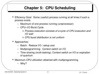
Chapter 5: CPU Scheduling • Basic Concepts • Scheduling Criteria • Scheduling Algorithms • Thread Scheduling • Multiple-Processor Scheduling • Linux Example
Objectives • To introduce CPU scheduling, which is the basis for multiprogrammed operating systems • To describe various CPU-scheduling algorithms • To discuss evaluation criteria for selecting a CPU-scheduling algorithm for a particular system
Basic Concepts • The objective of multiprogramming is to have some process running at all time, to Maximum CPU utilization. • CPU–I/O Burst Cycle – Process execution consists of a cycle of CPU execution and I/O wait • Process execution begins with a CPU burst that is followed by an I/O burst, which is followed by another CPU burst , then another I/O burst , and so on,.. The final CPU burst ends the process. • CPU burst distribution • large number of short CPU bursts and a small number of long CPU bursts. • An I/O –bound program has many short CPU bursts. • A CPU –bound program has few long CPU bursts.
CPU Scheduler • When the CPU becomes idle, the OS must Select from among the processes in memory that are ready to execute, and allocates the CPU to one of them. • The selection process is carried out by the short-term scheduler (CPU scheduler ). • CPU scheduling decisions may take place when a process: 1. Switches from running state to the waiting state(result of I/o request or wait for the termination of one of the child processes). 2. Switches from running state to ready state(interrupt). 3. Switches from waiting state to ready state(completion of I/O) 4. Terminates • Scheduling under 1 and 4 is nonpreemptive or cooperative. • All other scheduling is preemptive
Preemptive scheduling • Under nonpreemptive scheduling, once the CPU has been allocated to a process, the process keeps the CPU until it releases the CPU either by terminating or by switching to the waiting state. • Windows 95 and all subsequent versions of windows OS have used preemptive scheduling.
Dispatcher • The Dispatcher is the module that gives control of the CPU to the process selected by the short-term scheduler; this involves: • switching context • switching to user mode • jumping to the proper location in the user program to restart that program • It should be fast. • Dispatch latency – the time it takes for the dispatcher to stop one process and start another running
Scheduling Criteria • CPU utilization – keep the CPU as busy as possible. • Throughput – # of processes that complete their execution per time unit(10 processes/second) • Turnaround time – amount of time to execute a particular process(the interval from the time of submission of a process to the time of completion, waiting to get into memory, waiting in the ready queue, exciting on the CPU, doing I/O). • Waiting time – the amount of times a process has been waiting in the ready queue • Response time – amount of time it takes from when a request was submitted until the first response is produced, not output (for time-sharing environment)
Scheduling Algorithm Optimization Criteria • Max CPU utilization • Max throughput • Min turnaround time • Min waiting time • Min response time
First-Come, First-Served (FCFS) Scheduling • Jobs are scheduled in order of arrival • When a process enters the ready queue, its PCB is linked onto the tail of the queue. • When the CPU is free, it is allocated to the process at the head of the queue (the running process is then removed from the queue). • Disadvantages: • Non-preemptive : once the CPU is allocated to a process, the process keeps the CPU until it releases it, either by terminating or requesting I/O. • The average waiting time is often quite long.
P1 P2 P3 0 24 27 30 example ProcessBurst Time P1 24 P2 3 P3 3 • Suppose that the processes arrive in the order: P1 , P2 , P3 The Gantt Chart for the schedule is: • Waiting time for P1 = 0; P2 = 24; P3 = 27 • Average waiting time: (0 + 24 + 27)/3 = 17
P2 P3 P1 0 3 6 30 FCFS Scheduling (Cont) Suppose that the processes arrive in the order P2 , P3 , P1 • The Gantt chart for the schedule is: • Waiting time for P1 = 6;P2 = 0; P3 = 3 • Average waiting time: (6 + 0 + 3)/3 = 3 • Much better than previous case • Convoy effect as short processes go behind long process lower CPU and device utilization.
Shortest-Job-First (SJF) Scheduling • This algorithm Associates with each process the length of its next CPU burst. Use these lengths to schedule the process with the shortest time, if the next CPU bursts of two processes are the same, FCFS scheduling is used. • Two schemes: • Nonpreemptive – once CPU given to the process it cannot be preempted until completes its CPU burst • Preemptive – if a new process arrives with CPU burst length less than remaining time of current executing process, preempt. This scheme is known as the Shortest-Remaining-Time-First (SRTF)
P3 P2 P4 P1 3 9 16 24 0 Examples of SJF Example1: Process Arrival TimeBurst Time P10.0 6 P2 2.0 8 P34.0 7 P45.0 3 • SJF scheduling chart • Average waiting time = (3 + 16 + 9 + 0) / 4 = 7 • Compare with FCFS AWT=(0+6+14+21)/4=10.25
Shortest-Job-First (SJF) Scheduling Example2: ProcessArrival TimeBurst Time P1 0 7 P2 2 4 P3 4 1 P4 5 4 • Non preemptive SJF Average waiting time = (0 + 6 + 3 + 7)/4 = 4 P1 P3 P2 P4 4 5 2 0 7 8 12 16 P1‘s wating time = 0 P2‘s wating time = 6 P3‘s wating time = 3 P4‘s wating time = 7 P1(7) P2(4) P3(1) P4(4)
P1 P2 P3 P2 P4 P1 11 16 0 2 4 5 7 Shortest-Job-First (SJF) Scheduling Example3: ProcessArrival TimeBurst Time P1 0 7 P2 2 4 P3 4 1 P4 5 4 • Preemptive SJF(SRTF) Average waiting time = (9 + 1 + 0 +2)/4 = 3 P1‘s wating time = 9 P2‘s wating time = 1 P3‘s wating time = 0 P4‘s wating time = 2 P1(5) P1(7) P2(2) P2(4) P3(1) P4(4)
Shortest-Job-First (SJF) Scheduling • SJF is optimal – gives minimum average waiting time for a given set of processes • The difficulty is knowing the length of the next CPU request.
Priority Scheduling • A priority number (integer) is associated with each process • The CPU is allocated to the process with the highest priority (smallest integer highest priority in Unix but lowest in Java) • Equal-priority processes are scheduled in FCFS order. • Preemptive: preempt the CPU if the priority of the newly arrived process is higher than the priority of the currently running process. • Nonpreemptive : put the new process at the head of the ready queue. • SJF is a priority scheduling where priority is the predicted next CPU burst time • Problem Starvation – low priority processes may never execute • Solution Aging – as time progresses increase the priority of the process (for example : 1 every 15 minutes)
P1 P3 P2 P5 1 6 16 19 0 Priority Scheduling Example : ProcessBurst Timepriority P1 10 3 P2 1 1 P3 2 4 P4 1 5 p5 5 2 The AWT is (6 +0+ 16+18+1)/5 = 8.2 All arrived at time 0. The Gantt chart for the schedule is: P4 18
Priority Scheduling Example: Process arrival time Burst length Priority P1 0 10 3 P2 0 1 1 P3 0 2 4 P4 0 1 5 P5 3 5 2 • Gantt chart: Non-preemptive priority scheduling 0 1 11 16 18 19 • Gantt chart: Preemptive priority scheduling 0 1 3 8 16 18 19
Round Robin (RR) • Is designed especially for time-sharing systems. • Similar to FCFS, but it is Preemptive to enable the system to switch between processes. • Each process gets a small unit of CPU time (time quantum or time slice), usually 10-100 milliseconds. • The Ready queue is FIFO (new processes are added to the tail of the queue.) • The CPU scheduler picks the first process from the ready queue ,set a timer to interrupt after 1 time quantum, and dispatch the process.
Round Robin (RR) • One of two things will happen • The process may have a CPU burst of < 1 time quantum the process itself will release the CPU voluntarily. • The CPU burst of the currently running process > 1 time quantum the timer will go off and will cause an interrupt to the OS. a context switch will be executed, and the process will be put at the tail of the ready queue. • The CPU scheduler will then select the next process in the ready queue. • Typically, higher average turnaround than SJF, but better response
P1 P2 P3 P1 P1 P1 P1 P1 0 10 14 18 22 26 30 4 7 Round Robin (RR) Example1: Time quantum = 4 ProcessBurst Time P1 24 P2 3 P3 3 • The Gantt chart is: • AWT(6(10-4)+4+7)/3 = 5.66
P1 P2 P3 P4 P1 P3 P4 P1 P3 P3 0 20 37 57 77 97 117 121 134 154 162 Round Robin (RR) • Example2: • Time quantum = 20 ProcessBurst TimeWait Time P1 53 57 +24 = 81 P2 17 20 P3 68 37 + 40 + 17= 94 P4 2457 + 40 = 97 P1(13) P1(33) P1(53) 24 57 20 P2(17) P3(48) P3(28) P3(8) 40 37 17 P3(68) P4(4) 40 P4(24) 57 Average wait time = (81+20+94+97)/4 = 73
Round Robin (RR) • If there are n processes in the ready queue and the time quantum is q, then each process gets 1/n of the CPU time in chunks of at most q time units at once. No process waits more than (n-1)*q time units until its next time quantum. (Ex: 5 processes, TQ = 20 milliseconds, each process will get up to 20 milliseconds every 100 milliseconds. • The Performance of RR depends heavily on the size of the TQ. • TQ large FCFS • TQsmall TQ must be large (but not too large)with respect to context switch time, otherwise overhead is too high
Turnaround Time Varies With The Time Quantum The average TurnAroundTime of a set of process does not necessarily improve as the TQ size increase. The AVG TAT can be improved if most process finish their next CPU burst in a single time quantum.
Multilevel Queue • Processes are classified into different groups. • Each group have different response-time requirements different scheduling needs. • A multilevel queue scheduling algorithm partitions the Ready queue into separate queues:foreground (interactive)background (batch) • Each queue has its own scheduling algorithm • foreground – RR • background – FCFS • Scheduling must be done between the queues • Fixed priority preemptive scheduling; (i.e., serve all from foreground then from background). Possibility of starvation. • Time slice – each queue gets a certain amount of CPU time which it can schedule amongst its processes; i.e., 80% to foreground in RR, 20% to background in FCFS
Multilevel Feedback Queue • Implement multiple ready queues • Different queues may be scheduled using different algorithms • Just like multilevel queue scheduling, but assignments are not static • Multilevel feedback queue-scheduling algorithm allows a process to move between the various queues; aging can be implemented this way • Multilevel-feedback-queue scheduler defined by the following parameters: • number of queues • scheduling algorithms for each queue • method used to determine when to upgrade and downgrade a process • The most general CPU-scheduling algorithm. • The most complex algorithm.
Example of Multilevel Feedback Queue • Three queues: • Q0 – RR with time quantum 8 milliseconds • Q1 – RR time quantum 16 milliseconds • Q2 – FCFS • Scheduling • A new job enters queue Q0which is servedFCFS. When it gains CPU, job receives 8 milliseconds. If it does not finish in 8 milliseconds, job is moved to queue Q1. • At Q1 job is again served FCFS and receives 16 additional milliseconds. If it still does not complete, it is preempted and moved to queue Q2. • AT Q2 job is served FCFS only when queue 0 and queue 1 are empty.
Thread Scheduling • Distinction between user-level and kernel-level threads • On OSs that support them, it is the kernel-level threads-not processes- that are being scheduled by OS. • User-level threads are managed by a thread library and the kernel is unaware of them. • To run on CPU, the user level threads must be mapped to an associated kernel-level thread. It may use a lightweight process(LWP). contention scope: • one distinction between user-level and kernel-level threads lies in how they are scheduled.
Thread Scheduling • Many-to-one and many-to-many models, thread library schedules user-level threads to run on LWP. Known as process-contention scope (PCS) since scheduling competition takes place among threads belonging to the same process. • PCS is done according to preempt priority. • PTHREAD SCOPE PROCESS schedules threads using PCS scheduling. • Kernel thread scheduled onto available CPU is system-contention scope (SCS) – competition takes place among all threads in system • Systems using the one-to-one model schedule threads using only SCS. • PTHREAD SCOPE SYSTEM schedules threads using SCS scheduling.
Multiple-Processor Scheduling • CPU scheduling more complex when multiple CPUs are available • Different rules for homogeneous processors(Identical processors in terms of their functionality) or heterogeneous processors. • Asymmetric multiprocessing: • All scheduling decisions, I/O processing, and other system activities handled by a single processor – the master server. • The other processors execute only user code. • Simple because only one processor accesses the system data structures, reducing the need for data sharing. • Symmetric multiprocessing (SMP): • each processor is self-scheduling, all processes in common ready queue, or each has its own private queue of ready processes • Multiple processors try to access and update a common data structures. So, scheduler must be programmed carefully. • Must ensure that 2 processors don’t choose the same process.
Linux Scheduling • Linux Scheduler is a preemptive, priority-based algorithm with 2 separate priority ranges: • Two priority ranges: time-sharing and real-time • A real-time range from 0 to 99 Longer time quantum • A nice value ranging from 100 to 140 Shorter time quantum
Linux Scheduling • The kernel maintains a list of all runnable tasks in a runqueue data structure. • Each runqueue contains two priority arrays : • Active : contains all tasks with time remaining in their time slices • Expired : contains all expired tasks.
List of Tasks Indexed According to Priorities • The scheduler chooses the task with the highest priority from the active array for execution on the CPU. • When the active array is empty the 2 arrays are exchanged (the expired array becomes the active array, and vice versa).
Algorithm Evaluation • Deterministic modeling • takes a particular predetermined workload and defines the performance of each algorithm for that workload • More examples P: 214 • Simple and fast • Requires exact numbers for input and its answers apply only for those data • Queueingmodels • rate at which new processes arrive, ratio of CPU bursts to I/O times, distribution of CPU burst times and I/O burst times can be measured and then approximated or estimated • result is a mathematical formula describing it • From these it is possible to compute the average throughput, utilization, waiting time, and so on • difficult to work
Algorithm Evaluation • Simulations • run computer simulations of the different proposed algorithms • data to drive the simulation can be randomly generated • better alternative when possible is to generate trace tapes • expensive • Implementation • The only completely accurate way to evaluate a scheduling algorithm is to code it up, put it in the operating system, and see how it works. • high cost (coding and user reaction)
Conclusion • We’ve looked at a number of different scheduling algorithms. • Which one works the best is application dependent. • General purpose OS will use priority based, round robin, preemptive • Real Time OS will use priority, no preemption.