Download
1 / 54
540 likes | 577 Views
Discover the fundamental concepts of statistics, from organizing and interpreting data to drawing conclusions about populations. Learn about descriptive statistics, inferential statistics, parameters, sampling error, and frequency distributions. Explore various tools like frequency tables, histograms, and stem-and-leaf plots to analyze data effectively.

E N D
Introduction to Statistics I. What are Statistics? • Procedures for organizing, summarizing, and interpreting information • Standardized techniques used by scientists • Vocabulary & symbols for communicating about data • A tool box • How do you know which tool to use? (1) What do you want to know? (2) What type of data do you have? • Two main branches: • Descriptive statistics • Inferential statistics
Two Branches of Statistical Methods • Descriptive statistics • Techniques for describing data in abbreviated, symbolic fashion • Inferential statistics • Drawing inferences based on data. Using statistics to draw conclusions about the population from which the sample was taken.
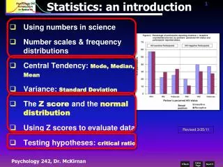
Descriptive vs Inferential A. Descriptive Statistics: Tools for summarizing, organizing, simplifying data Tables & Graphs Measures of Central Tendency Measures of Variability Examples: Average rainfall in Richmond last year Number of car thefts in IV last quarter Your college G.P.A. Percentage of seniors in our class B.Inferential Statistics: Data from sample used to draw inferences about population Generalizing beyond actual observations Generalize from a sample to a population
Populations and Samples • A parameter is a characteristic of a population • e.g., the average height of all Americans. • A statistics is a characteristic of a sample • e.g., the average height of a sample of Americans. • Inferential statistics infer population parameters from sample statistics • e.g., we use the average height of the sample to estimate the average height of the population
Symbols and Terminology: Parameters = Describe POPULATIONS Greek letters 2 Statistics = Describe SAMPLES Englishletters s2sr Sample will not be identical to the population So, generalizations will have some error Sampling Error = discrepancy between sample statistic and corresponding popl’n parameter
Statistics are Greek to me! Statistical notation: X = “score” or “raw score” N = number of scores in population n = number of scores in sample Quiz scores for 5 Students: X = Quiz score for each student
Statistics are Greek to me! X = Quiz score for each student Y = Number of hours studying Summation notation: “Sigma” = ∑ “The Sum of” ∑X = add up all the X scores ∑XY = multiply X×Y then add
Descriptive Statistics Numerical Data Properties Central Variation Shape Tendency Mean Range Skewness Modes Median Interquartile Range Mode Standard Deviation Variance
Ordering the Data: Frequency Tables • Three types of frequency distributions (FDs): • (A) Simple FDs • (B) Relative FDs • (C) Cumulative FDs • Why Frequency Tables? • Gives some order to a set of data • Can examine data for outliers • Is an introduction to distributions
QUIZ SCORES (N = 30) 10 7 6 5 3 9 7 6 5 3 9 7 6 4 3 8 7 5 4 2 8 6 5 4 2 8 6 5 4 1 Simple Frequency Distribution of Quiz Scores (X) A. Simple Frequency Distributions f = N = 30
Relative Frequency Distribution Quiz Scores f=N=30 ==
Cumulative Frequency Distribution __________________________________________________ Quiz Score f p % cf c% __________________________________________________ __________________________________________________ = 30 =1.0= 100%
Grouped Frequency Tables Assign fs to intervals Example: Weight for 194 people Smallest = 93 lbs Largest = 265 lbs f = N = 194
Graphs of Frequency Distributions • A picture is worth a thousand words! • Graphs for numerical data: Stem & leaf displays Histograms Frequency polygons • Graphs for categorical data Bar graphs
Cross between a table and a graph Like a grouped frequency distribution on its side Easy to construct Identifies each individual score Each data point is broken down into a “stem” and a “leaf.” Select one or more leading digits for the stem values. The trailing digit(s) becomes the leaves First, “stems” are aligned in a column. Record the leaf for every observation beside the corresponding stem value Making a Stem-and-Leaf Plot
6 4 3 8 3 2 8 5 1 2 3 2 Stem and Leaf / Histogram Stem Leaf 2 1 3 4 3 2 2 3 6 4 3 8 8 5 2 5 By rotating the stem-leaf, we can see the shape of the distribution of scores. Leaf Stem 2 3 4 5
Histograms • Histograms
Histograms • f on y axis (could also plot p or % ) • X values (or midpoints of class intervals) on x axis • Plot each f with a bar, equal size, touching • No gaps between bars
Frequency Polygons • Frequency Polygons • Depicts information from a frequency table or a grouped frequency table as a line graph
Frequency Polygon A smoothed out histogram Make a point representing f of each value Connect dots Anchor line on x axis Useful for comparing distributions in two samples (in this case, plot p rather than f )
Frequency tables, histograms & polygons describe how the frequencies are distributed Distributions are a fundamental concept in statistics One peak Unimodal Two peaks Bimodal Shapes of Frequency Distributions
Normal and Bimodal Distributions (1) Normal Shaped Distribution • Bell-shaped • One peak in the middle (unimodal) • Symmetrical on each side • Reflect many naturally occurring variables (2) Bimodal Distribution • Two clear peaks • Symmetrical on each side • Often indicates two distinct subgroups in sample
Symmetrical vs. Skewed Frequency Distributions • Symmetrical distribution • Approximately equal numbers of observations above and below the middle • Skewed distribution • One side is more spread out that the other, like a tail • Direction of the skew • Positive or negative (right or left) • Side with the fewer scores • Side that looks like a tail
Symmetric Skewed Right Skewed Left Symmetrical vs. Skewed
Skewed Frequency Distributions • Positively skewed • AKA Skewed right • Tail trails to the right • *** The skew describes the skinny end ***
Skewed Frequency Distributions • Negatively skewed • Skewed left • Tail trails to the left
Bar Graphs • For categorical data • Like a histogram, but with gaps between bars • Useful for showing two samples side-by-side
Central Tendency • Give information concerning the average or typical score of a number of scores • mean • median • mode
Central Tendency: The Mean • The Mean is a measure of central tendency • What most people mean by “average” • Sum of a set of numbers divided by the number of numbers in the set
Central Tendency: The Mean Arithmetic average: Sample Population
Central Tendency: The Mean • Important conceptual point: • The mean is the balance point of the data in the sense that if we took each individual score (X) and subtracted the mean from them, some are positive and some are negative. If we add all of those up we will get zero.
Central Tendency:The Median • Middlemost or most central item in the set of ordered numbers; it separates the distribution into two equal halves • If odd n, middle value of sequence • if X = [1,2,4,6,9,10,12,14,17] • then 9 is the median • If even n, average of 2 middle values • if X = [1,2,4,6,9,10,11,12,14,17] • then 9.5 is the median; i.e., (9+10)/2 • Median is not affected by extreme values
Median vs. Mean • Midpoint vs. balance point • Md based on middle location/# of scores • based on deviations/distance/balance • Change a score, Md may not change • Change a score, will always change
Central Tendency: The Mode • The mode is the most frequently occurring number in a distribution • if X = [1,2,4,7,7,7,8,10,12,14,17] • then 7 is the mode • Easy to see in a simple frequency distribution • Possible to have no modes or more than one mode • bimodal and multimodal • Don’t have to be exactly equal frequency • major mode, minor mode • Mode is not affected by extreme values
When to Use What • Mean is a great measure. But, there are time when its usage is inappropriate or impossible. • Nominal data: Mode • The distribution is bimodal: Mode • You have ordinal data: Median or mode • Are a few extreme scores: Median
Mean Mean Mean Median Mode Mode Mode Median Median Symmetric (Not Skewed) Positively Skewed Negatively Skewed Mean, Median, Mode
Measures of Central Tendency Overview Central Tendency Mode Mean Median Midpoint of ranked values Most frequently observed value
Class Activity • Complete the questionnaires • As a group, analyze the classes data from the three questions you are assigned • compute the appropriate measures of central tendency for each of the questions • Create a frequency distribution graph for the data from each question
Variability • Variability • How tightly clustered or how widely dispersed the values are in a data set. • Example • Data set 1: [0,25,50,75,100] • Data set 2: [48,49,50,51,52] • Both have a mean of 50, but data set 1 clearly has greater Variability than data set 2.
Variability: The Range • The Range is one measure of variability • The range is the difference between the maximum and minimum values in a set • Example • Data set 1: [1,25,50,75,100]; R: 100-1 +1 = 100 • Data set 2: [48,49,50,51,52]; R: 52-48 + 1= 5 • The range ignores how data are distributed and only takes the extreme scores into account • RANGE = (Xlargest – Xsmallest) + 1
Quartiles • Split Ordered Data into 4 Quarters • = first quartile • = second quartile= Median • = third quartile 25% 25% 25% 25%
Variability: Interquartile Range • Difference between third & first quartiles • Interquartile Range = Q3 - Q1 • Spread in middle 50% • Not affected by extreme values
Standard Deviation and Variance • How much do scores deviate from the mean? • deviation = • Why not just add these all up and take the mean? = 2
Standard Deviation and Variance • Solve the problem by squaring the deviations! = 2 Variance =
Standard Deviation and Variance • Higher value means greater variability around • Critical for inferential statistics! • But, not as useful as a purely descriptive statistic • hard to interpret “squared” scores! • Solution un-square the variance! Standard Deviation =
Variability: Standard Deviation • The Standard Deviation tells us approximately how far the scores vary from the mean on average • estimate of average deviation/distance from • small value means scores clustered close to • large value means scores spread farther from • Overall, most common and important measure • extremely useful as a descriptive statistic • extremely useful in inferential statistics The typical deviation in a given distribution