Download
1 / 13
130 likes | 244 Views
Optimal Electricity Supply Bidding by Markov Decision Process. Presentation Review By: Feng Gao, Esteban Gil, & Kory Hedman IE 513 Analysis of Stochastic Systems Professor Sarah Ryan March 28, 2005. Authors: Haili Song, Chen-Ching Liu, Jacques Lawarree, & Robert Dahlgren. Outline.

E N D
Optimal Electricity Supply Bidding by Markov Decision Process Presentation Review By: Feng Gao, Esteban Gil, & Kory Hedman IE 513 Analysis of Stochastic Systems Professor Sarah Ryan March 28, 2005 Authors: Haili Song, Chen-Ching Liu, Jacques Lawarree, & Robert Dahlgren
Outline • Summary of the previous presentation • Model Validation • Implementation and case study • Description of Examples • Summary
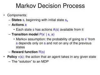
Summary of previous presentation • Introduction • Electric Market is now Competitive • GenCos Bid on Demand • Purpose • MDP Used to Determine Optimal Bidding Strategy • Problem Formulation • Transition Probability Determined by Current State, Subsequent State, & Decision Made • 7 Variables to Define a State • Aggregation Used to Limit Dimensionality Problems • Model Overview • 7 Day Planning Horizon • Objective is to Maximize Summation of Expected Reward • Value Iteration
Value Iteration Discussion • V (i, T+1): Total Expected Reward in T+1 Remaining Stages from State I • At the last stage T = 0 • Value Iteration (Backward Induction) • Ignore discount factor • The immediate reward is dependent on the initial state, following state and decision a
Model Overview Clarification • Sum of all Scenarios S that result in a given spot price, cleared quantity, and production limit. • Prob to Move from State i to j given decision a = [Prob (that the spot price, production level are correct and load forecast = demand)*prob(of having the proper load forecast)] • Resulting Spot Price can be dependent on Decision a if the bidder has market power
Model Validation • For model validation: • Accumulate actual data and observations from the market over a period of time (e.g. 1 year) • Market data set provides the actual scenarios • Relationship between estimated by the BIDS representation r(i,j,a) and actual rewards w(i,j,a) can be analyzed by linear regression.
Case Study • 3 suppliers: GenCoA, GenCoB, and GenCoC, all bidding in the spot market • GenCoA is the decision maker using the Markov Decision Process technique • GenCoA: 1 generating unit • GenCoB: 2 generating units • GenCoC: 2 generating units • Planning Horizon: 7 days (bid decision for next day considers the entire week ahead
Case Study • GenCoA makes a decision from a set of pre-specified decision options • GenCoA does not know exactly how GenCoB and GenCoC are going to bid • But their individual bidding behavior is modeled by bid prices, quantities and the associated probabilities based on GenCoA’s knowledge and information • Transition probabilities and rewards are calculated using algorithm described in previous presentation
Two Basic Market Situations • EXAMPLE 1: • Decision-maker has a production limit over the planning horizon • Decision-maker does not have market power (perfect competition) • Optimal strategy is time dependent due to the production limit • In some states the optimal decision is not to sell, but to save the resources for more profitable days
Two Basic Market Situations • EXAMPLE 2: • Decision-maker has market power: it can manipulate the bid to influence the spot price • Decision-maker has no production limit • Decision-maker makes the bidding decision to maximize the expected reward over the planning horizon • Daily maximum strategy is time independent: decision-maker makes the same decision as long as the system is in the same state • BIDS value iteration is time dependent: it takes into account how current biddings affect future spot prices
Comparison of Two Cases • Without market power, bidder is concerned with saving resources for more expensive periods • With market power, bidder is concerned with properly influencing the future spot price to maximize profit • Knowing whether the bidder has market power or not is crucial since the relationship between spot prices and decisions would depend on each other
Summary • Model Overview • 7 Day Planning Horizon • Objective is to Maximize Summation of Expected Reward • Value Iteration • Model Validation • Comparison of Predicted and Actual Results (by linear regression) • Implementation and case study • Three GenCos, GenCo A is the Decision Maker • 5 Generators among the 3 GenCos • Description of 2 Examples: • Production Limit without Market Power • Market Power without Production Limit • Next Time: Presentation and Discussion of Results and Conclusions