Fast 3D Target-Oriented Reverse Time Datuming
This presentation outlines the advancements in reverse time migration (RTM) and target-oriented reverse time datuming (RTD) aimed at improving subsalt imaging and reducing defocusing artifacts in seismic data. The methodology utilizes both 2D and 3D SEG/EAGE salt models alongside field data to demonstrate the effectiveness of RTD in enhancing resolution and computational efficiency. Numerical tests show that redatumed data allows for improved migration velocity analysis (MVA) while maintaining accuracy and reducing computational costs. Key findings include enhanced image quality and the ability to bypass overburden effects.
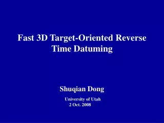

Fast 3D Target-Oriented Reverse Time Datuming
E N D
Presentation Transcript
Fast 3D Target-Oriented Reverse Time Datuming Shuqian Dong University of Utah 2 Oct. 2008
Outline • Motivation • Theory • Numerical Tests 2-D SEG/EAGE salt model 3-D SEG/EAGE salt model 3-D field data • Conclusions Motivation Numerical Tests Theory Conclusions
Motivation Numerical Tests Theory Conclusions Outline • Motivation • Theory • Numerical Tests 2-D SEG/EAGE salt model 3-D SEG/EAGE salt model 3-D field data • Conclusions
km/s Velocity model 0 0 0 Common shot gather 4.5 Time (s) z (km) z (km) 1.5 2.0 4.0 2.0 x (km) x (km) x (km) 8.0 8.0 8.0 0 0 0 KM image Problem: Defocusing: lower resolution, distorted image Multiples: image artifacts. Reason: KM: high frequency approximation. Motivation Numerical Tests Theory Conclusions Motivation Solutions?
RTM image Velocity model KM image Motivation Numerical Tests Theory Conclusions Motivation Solutions: • Reverse time migration: solving two-way wave equation • Target-oriented reverse time datuming: • solving two-way wave equation to bypass overburden Luo, 2002: target-oriented RTD Luo and Schuster, 2004: bottom-up strategy
RTD • Complex structures cause defocusing effects • RTD can reduce defocusing effects • RTM is computationally expensive • RTD + Kirchhoff = accurate + cheap Motivation Numerical Tests Theory Conclusions Motivation
Motivation Numerical Tests Theory Conclusions Motivation • Reduce defocusing effects for subsalt imaging • Closer to the target: better resolution • Bottom-up strategy: computational efficiency • Redatumed data can be used for least squares • migration and migration velocity analysis (MVA)
Motivation Numerical Tests Theory Conclusions Outline • Motivation • Theory • Numerical Tests 2-D SEG/EAGE salt model 3-D SEG/EAGE salt model 3-D field data • Conclusions
Motivation Numerical Tests Theory Conclusions Theory Reverse time datuming d(s|r) S R x’’ x’
d(s|x’’) g*(r|x”) d(s|r) d(s|x”)= Motivation Numerical Tests Theory Conclusions Theory Reverse time datuming S R x’’ x’
g*(r|x”) d(s|r) d(s|x”)= d(x’|x’’) Motivation Numerical Tests Theory Conclusions Theory Reverse time datuming S R d(x’|x”)=g*(s|x’) d(s|x”) x’’ x’
Real source number on surface: 10 Virtual source number on datum: 3 Motivation Numerical Tests Theory Conclusions Theory Calculate Green’s functions VSP (source on surface) Green’s functions: 10
Real source number on surface: 10 Virtual source number on datum: 3 VSP (source on surface) Green’s functions: 10 Motivation Numerical Tests Theory Conclusions Theory Calculate Green’s functions Reciprocity: RVSP=VSP RVSP (source on datum) Green’s functions: 3
Reciprocity: RVSP =>VSP Green’s functions: FFT: time domain => frequency domain Crosscorrelation: Green’s functions with original data IFFT: frequency domain => time domain Redatumed data Motivation Numerical Tests Theory Conclusions Workflow FD: Compute RVSP Green’s functions Original data: FFT: time domain =>frequency domain
Motivation Numerical Tests Theory Conclusions Outline • Motivation • Theory • Numerical Tests 2-D SEG/EAGE salt model 3-D SEG/EAGE salt model 3-D field data • Conclusions
km/s Velocity model 0 0 0 0 4.5 Time (s) Time (s) Time (s) z (km) 1.5 2.0 4.0 4.0 4.0 x (km) x (km) x (km) x (km) 8.0 8.0 8.0 8.0 0 0 0 0 Motivation Numerical Tests Theory Conclusions 2D SEG/EAGE Test RVSP Green’s function True CSG at datum Redatumed CSG
km/s Velocity model 0 0 0 0 4.5 z (km) z (km) z (km) z (km) 1.5 2.0 2.0 2.0 2.0 x (km) x (km) x (km) x (km) 8.0 8.0 8.0 8.0 0 0 0 0 KM image RTM image Motivation Numerical Tests Theory Conclusions 2D SEG/EAGE Test KM of redatumed data
Motivation Numerical Tests Theory Conclusions Outline • Motivation • Theory • Numerical Tests 2-D SEG/EAGE salt model 3-D SEG/EAGE salt model 3-D field data • Conclusions
km/s 4.5 0 x (km) 3.5 0 1.5 Z (km) 2.0 0 y (km) 2 Motivation Numerical Tests Theory Conclusions 3D SEG/EAGE test Velocity model SSP geometry: 1700 shots 1700 receivers Datum depth: 1.5 km RVSP Green’s functions: 850 shots 1700 receivers
Original CSG RVSP Green’s function 0 0 0 0 Time (s) Time (s) Time (s) Time (s) 2.5 2.5 2.5 2.5 Redatumed CSG True CSG at datum y (km) y (km) y (km) y (km) 3.5 3.5 3.5 3.5 0 0 0 0 Motivation Numerical Tests Theory Conclusions 3D SEG/EAGE test
KM of RTD data x (km) x (km) 0 0 3.5 3.5 0 0 Z (km) Z (km) 2.0 2.0 0 0 y (km) y (km) 2 2 KM of original data Motivation Numerical Tests Theory Conclusions 3D SEG/EAGE test
KM of original data KM of redatumed data 0 0 0 z (km) z (km) z (km) 2.0 2.0 2.0 3.5 3.5 3.5 x (km) x (km) x (km) 0 0 0 Velocity model Motivation Numerical Tests Theory Conclusions 3D SEG/EAGE test ( Inline No. 41 )
0 0 0 z (km) z (km) z (km) 2.0 2.0 2.0 3.5 3.5 3.5 x (km) x (km) x (km) 0 0 0 Motivation Numerical Tests Theory Conclusions 3D SEG/EAGE test KM of original data KM of redatumed data Velocity model ( Inline No. 101 )
0 0 0 z (km) z (km) z (km) 2.0 2.0 2.0 2.0 2.0 2.0 y (km) y (km) y (km) 0 0 0 Motivation Numerical Tests Theory Conclusions 3D SEG/EAGE test KM of original data KM of redatumed data Velocity model ( Crossline No. 161 )
0 0 0 z (km) z (km) z (km) 2.0 2.0 2.0 2.0 2.0 2.0 y (km) y (km) y (km) 0 0 0 Motivation Numerical Tests Theory Conclusions 3D SEG/EAGE test KM of original data KM of redatumed data Velocity model ( Crossline No. 201 )
0 0 0 y (km) y (km) y (km) 2.0 2.0 2.0 3.5 3.5 3.5 x (km) x (km) x (km) 0 0 0 Motivation Numerical Tests Theory Conclusions 3D SEG/EAGE test KM of original data KM of redatumed data Velocity model ( depth: z=1.4 km )
0 0 0 y (km) y (km) y (km) 2.0 2.0 2.0 3.5 3.5 3.5 x (km) x (km) x (km) 0 0 0 Motivation Numerical Tests Theory Conclusions 3D SEG/EAGE test KM of original data KM of redatumed data Velocity model ( depth: z=1.5 km )
Motivation Numerical Tests Theory Conclusions Outline • Motivation • Theory • Numerical Tests 2-D SEG/EAGE salt model 3-D SEG/EAGE salt model 3-D field data • Conclusions
Interval velocity model km/s 0 5.5 Z (km) 8.0 0 y (km) 12 x (km) 6.0 0 1.5 Motivation Numerical Tests Theory Conclusions 3D Field Data Test OBC geometry: 50,000 shots 180 receivers per shot Datum depth: 1.5 km RVSP Green’s functions: 5,000 shots 180 receivers per shot
Redatumed CSG Original CSG 0 0 Time (s) Time (s) 6.0 6.0 y (km) y (km) 4.5 4.5 0 0 Motivation Numerical Tests Theory Conclusions 3D Field Data Test
x (km) 0 12 KM of original data 0 Z (km) 8 KM of redatumed data 0 0 y (km) 5 Z (km) 8 0 12 y (km) x (km) 5 0 Motivation Numerical Tests Theory Conclusions 3D Field Data Test KM of RTD data
0 0 Z (km) Z (km) 8.0 8.0 0 0 X (km) X (km) 12 12 Motivation Numerical Tests Theory Conclusions 3D Field Data Test ( Inline No. 21 ) KM of original data KM of RTD data
0 0 Z (km) Z (km) 8.0 8.0 0 0 X (km) X (km) 12 12 Motivation Numerical Tests Theory Conclusions 3D Field Data Test ( Inline No. 41 ) KM of original data KM of RTD data
0 0 Z (km) Z (km) 8.0 8.0 0 0 X (km) X (km) 12 12 Motivation Numerical Tests Theory Conclusions 3D Field Data Test ( Inline No. 61 ) KM of original data KM of RTD data
0 0 Z (km) Z (km) 8.0 8.0 0 0 Y (km) Y (km) 5.0 5.0 Motivation Numerical Tests Theory Conclusions 3D Field Data Test ( Crossline No. 41 ) KM of original data KM of RTD data
0 0 Z (km) Z (km) 8.0 8.0 0 0 Y (km) Y (km) 5.0 5.0 Motivation Numerical Tests Theory Conclusions 3D Field Data Test ( Crossline No. 61 ) KM of original data KM of RTD data
0 0 Z (km) Z (km) 8.0 8.0 0 0 Y (km) Y (km) 5.0 5.0 Motivation Numerical Tests Theory Conclusions 3D Field Data Test ( Crossline No. 81 ) KM of original data KM of RTD data
0 0 Y (km) Y (km) 5.0 5.0 0 0 X (km) X (km) 12 12 Motivation Numerical Tests Theory Conclusions 3D Field Data Test ( Depth 2.0 km ) KM of original data KM of RTD data
0 0 Y (km) Y (km) 5.0 5.0 0 0 X (km) X (km) 12 12 Motivation Numerical Tests Theory Conclusions 3D Field Data Test ( Depth 2.5 km ) KM of original data KM of RTD data
0 0 Y (km) Y (km) 5.0 5.0 0 0 X (km) X (km) 12 12 Motivation Numerical Tests Theory Conclusions 3D Field Data Test ( Depth 4.0 km ) KM of original data KM of RTD data
Motivation Numerical Tests Theory Conclusions Computational Costs
Motivation Numerical Tests Theory Conclusions Outline • Motivation • Theory • Numerical Tests 2-D SEG/EAGE salt model 3-D SEG/EAGE salt model 3-D field data • Conclusions
Motivation Numerical Tests Theory Conclusions Conclusions • 2-D numerical test KM of RTD achieved image quality comparable to RTM at much lower cost. • 3-D numerical test 3-D RTD is implemented for synthetic and GOM data at acceptable computational cost; Apparent improvements in mage quality are achieved compared to KM image of original data. • Future application Subsalt least suqares migration and migration velocity analysis
Acknowledgements • Dr. Gerard Schuster and my committee members: Dr. Michael Zhdanov, Dr. Richard D. Jarrard for their advice and constructive criticism; • UTAM friends: • Dr. Xiang Xiao, Weiping Cao, and Chaiwoot Boonyasiriwat for their help on my thesis research; • Ge Zhang for his experiences on field data processing; • Dr. Sherif Hanafy, Shengdong Liu, Naoshi Aoki and all other UTAM members for their support in my life and work; • CHPC for the computation support.
km/s Velocity model 0 0 0 0 Common shot gather 4.5 Time (s) z (km) z (km) z (km) 1.5 2.0 2.0 2.0 4.0 x (km) x (km) x (km) x (km) 8.0 8.0 8.0 8.0 0 0 0 0 KM image RTM image Motivation Numerical Tests Theory Conclusions Motivation
Motivation Numerical Tests Theory Conclusions Theory Traditional reverse time datuming d(s|r) S R x’’ x’
d(s|x’’) g*(r|x”) d(s|r) d(s|x”)= Motivation Numerical Tests Theory Conclusions Theory Reverse time Datuming S R x’’ x’
g*(r|x”) d(s|r) d(s|x”)= d(x’|x’’) Motivation Numerical Tests Theory Conclusions Theory Reverse time Datuming S R d(x’|x”)=g*(s|x’) d(s|x”) x’’ x’
Motivation Numerical Tests Theory Conclusions Theory Target-oriented RTD (Luo , 2006)