EE 6358 Computer vision Image Filtering
EE 6358 Computer vision Image Filtering. By Srividya Varanasi Graduate Student Dept of Electrical Engineering Fall 2005. Need for image filtering. Remove noise Sharpen contrast Highlight contours in images. Basic terminology.

EE 6358 Computer vision Image Filtering
E N D
Presentation Transcript
EE 6358 Computer vision Image Filtering By Srividya Varanasi Graduate Student Dept of Electrical Engineering Fall 2005
Need for image filtering • Remove noise • Sharpen contrast • Highlight contours in images
Basic terminology The Spatial, Frequency and Time domains: Time domain applies to signals which are represented only in 1D Ex: Audio signals The spatial domain describes a 2D signal Ex: Image Both these domains can be converted to frequency domain
Linearity: 1D Convolution: 2D convolution:
Histogram Modification Purpose for histogram modification: • To sharpen the contrast of an image Reasons for poor contrast: • Many images contain unevenly distributed gray values. It is common to find the intensities to lie within a small range, resulting in poor contrast.
Definition:. If an image has a histogram of pixel intensities that has been highly skewed toward darker levels, detail is often imperceptible in the darker regions when such an image is viewed on a conventional display with only 8-bit pixels. Histogram modification can alleviate this problem by rescaling the original image so that the histogram of pixel intensities follows some preferred form.
Method of histogram modification: Histogram modification is a method of stretching the contrast of the image by Uniformly redistributing the gray values. An example of histogram modification is image scaling, in which pixels in range [a,b] are expanded to fill the range [z1,zk]
The formula for mapping a pixel value ‘z’ in the original range into a pixel value z’ in the new range is given by: Eqn 1.1
Drawbacks of image scaling: • The histogram stretched according to equation 1.1 has gaps between bins. • Often artifacts appearby using this method
Alternate methods of histogram modification: • If the desired gray value distribution is known ahead of time then If Pi be the number of pixels at level zi in the original histogram qi the number of pixels at level zi in the desired histogram We begin at the left end of the original histogram and find K1 such that
The pixels at levels z1 , z2 …..,zk1-1 map to level z1 in the new image. Next , find gray value k2 such that The next range of pixel values zk1 , zk2 …..,zk2-1 map to level z2 in the new image. This procedure is repeated until all gray values in original histogram have been added.
Original picture After histogram modification
Common types of noise • Salt and pepper noise • Impulse noise • Gaussian noise
Salt n pepper noise: Salt and pepper noise contains random occurrences of both black and white intensity values.
Original image Image with noise Salt and pepper noise
Impulse noise: • Impulse noise is noise of short duration and high energy. • It mostly occurs in over the air transmission such as satellite transmission. • Common sources of impulse noise are lightening, industrial machines, high voltage power lines.
Original image Image affected by impulse noise
Gaussian Noise: • Gaussian noise has equal energy at all frequencies. • While the frequency distribution may be the same, the amplitude near zero are more common, and extreme values are less common.
Original image image affected by Gaussian noise
Linear Filters • Good for removing Gaussian noise as well as other types of noise • Is implemented using weighted sum of pixels in successive windows.
1.Mean Filter • It is implemented by a local averaging operation where the value of each pixel is replaced by the average of all the values in the local neighborhood. 19 X
Salt n pepper noise 3X3 mean filter 5X5 mean filter
Drawbacks of Mean Filter These examples illustrate the two main problems with mean filtering, which are: • A single pixel with a very unrepresentative value can significantly affect the mean value of all the pixels in its neighborhood. • When the filter neighborhood straddles an edge, the filter will interpolate new values for pixels on the edge and so will blur that edge. This may be a problem if sharp edges are required in the output.
Median Filter The problems encountered by using a mean filter are tackled by the median filter, which is often a better filter for reducing noise than the mean filter, but it takes longer to compute.
Like the mean filter , the median filter considers each pixel in the image in turn and looks at its nearby neighbors to decide whether or not it is representative of its surroundings. Instead of simply replacing the pixel value with the mean of neighboring pixel values, it replaces it with the median of those values. • The median is calculated by first sorting all the pixel values from the surrounding neighborhood into numerical order and then replacing the pixel being considered with the middle pixel value. (If the neighborhood under consideration contains an even number of pixels, the average of the two middle pixel values is used.) Figure 1 illustrates an example calculation.
Gaussian Smoothing Filter • They are a class of linear smoothing filters with the weights chosen according to the shape of a Gaussian function. • It is very good filter for removing noise drawn from a normal distribution.
The 2D zero-mean discrete Gaussian function used for processing images is as given A plot of this function is as shown in the figure
Properties of Gaussian filters: • Amount of smoothing performed will be same in all directions, since Gaussian functions are rotationally symmetric. • Gaussian filter smooths by replacing each image pixel with a weighted average of the neighboring pixels such that the weight given to a neighbor decreases monotonically with distance from central pixel. This property helps in retaining the edges.
The width and hence the degree of smoothing, of a Gaussian filter is parameterized by standard deviation. The larger the deviation wider the Filter and the greater the smoothing and vice versa • Since Gaussian functions are separable ,large filters can be implemented very efficiently. Slide 32
Fast detection and impulsive noise removal in images Review of impulse noise: Impulse noise is noise of short duration and high energy. It mostly occurs in over the air transmission such as satellite transmission. Common sources of impulse noise are lightening, industrial machines, high voltage power lines. Reference: IEEE Transactions on image processing VOL 10 No.1 Jan 2001
Noise detection algorithm: The detection of corrupted signals in the image is performed by calculating the distances between the central pixels and its neighbors and counting the number of neighbors whose distance to the central pixel is not exceeding a predefined threshold . • The number of pixels which are close enough to the pixel under consideration serves as an indicator whether the pixel is corrupted by impulse noise or not
The central pixel in the filtering window is detected as unaffected by impulse noise if there are m neighbors in the window, which are close enough. • The closeness is defined by a distance parameter d. Otherwise, it will be replaced by the vector median of samples in the window.
Advantages of this method: • The main advantages of this technique is its simplicity and enormous computational speed. • Many well known filters introduce too much smoothing, which results in blurring of the output image. This undesired property is caused by unnecessary filtering of the noise-free samples that should be passed to the filter output without any change.