Download
1 / 26
260 likes | 280 Views
Learn confidence intervals, margin of error, interval estimators, and sample size in simulating stochastic variables.

E N D
Al-Imam Mohammad Ibn Saud University CS433Modeling and SimulationLecture 16 Output Analysis Large-Sample Estimation Theory Dr. Anis Koubâa 30 May 2009
Goals of Today • Understand the problem of confidence in simulation results • Learn how to determine of range of value with a certain confidence a certain stochastic simulation result • Understand the concept of • Margin of Error • Confidence Interval with a certain level of confidence
Reading • Required • Lemmis Park, Discrete Event Simulation - A First Course, Chapter 8: Output Analysis • Optional • Harry Perros, Computer Simulation Technique - The Definitive Introduction, 2007Chapter 5
Problem Statement • For a deterministic simulation model one run will be sufficient to determine the output. • A stochastic simulation model will not give the same result when run repetitively with independent random seed. • One run is not sufficient to obtain confident simulation results from one sample. • Statistical Analysis of Simulation Result: multiple runs to estimate the metric of interest with a certain confidence
Example: • Stoachatsic Simulation resultsmayvaryfrom one run/replication to another • Simulation results depends on three factors: • The seed of the RNG • Number of samples/size of samples • Simulation time • Objective • For a given large sample output, determine what is the mean value with a certain confidence on the result.
What types of parameters to estimate? • In general, a stochastic variable is described by their probability distributions and parameters. • For quantitative random variables: mean mand variance s. • For a binomial random variables: success probability p. • If the values of parameters are unknown, we make inferences about them using sample information.
How to express the confidence? • Simulation results must be expressed with a certain confidence. • The confidence needs the following parameters • Confidence Level: 99%, 98%, 95% or 90% • Variance: the variance of the simulation results • Sample Size: the number of simulation results under study • There are two ways: • Margin of Error: The maximum error of estimation. • Confidence interval: The interval where most of the simulation results lie.
The Margin of Error • Margin of error: The maximum error of estimation, calculated as
Estimating Means and Proportions • For a quantitative population, • For a binomial population,
Example 1 • A homeowner randomly samples 64 homes similar to his own and finds that the average selling price is 252,000 SAR with a standard deviation of 15,000 SAR. Question: Estimate the average selling price for all similar homes in the city.
Example 2 A quality control technician wants to estimate the proportion of soda bottles that are under-filled. He randomly samples 200 bottles of soda and finds 10 under-filled cans. What is the estimation of the proportion of under-filled cans?
Interval Estimators Confidence Interval
Parameter 1.96SE Confidence Interval • “Fairly sure” means “with high probability”, measured using the confidence coefficient, 1-a. Usually, 1-a = 0.90, 0.95, 0.98, 0.99 • Suppose 1-a = 0.95 and that the estimator has a normal distribution.
To Change the Confidence Level • To change to a general confidence level, 1-a, pick a value of z that puts area 1-a in the center of the z-distribution (i.e. Normal Distribution N(0,1). 100(1-a)% Confidence Interval: Estimator za/2SE
Confidence Intervals for Means and Proportions • For a quantitative population • For a binomial population
Example 1 • A random sample of n = 50 males showed a mean average daily intake of dairy products equal to 756 grams with a standard deviation of 35 grams. • Find a 95% confidence interval for the population average m.
Example 1 • Find a 99% confidence interval for m, the population average daily intake of dairy products for men. The interval must be wider to provide for the increased confidence that is does indeed enclose the true value of m.
Example 2 • Of a random sample of n = 150 college students, 104 of the students said that they had played on a soccer team during their K-12 years. • Estimate the proportion of college students who played soccer in their youth with a 98% confidence interval.
Choosing the Sample Size • The total amount of relevant information in a sample is controlled by two factors: - The sampling planor experimental design: the procedure for collecting the information - The sample size n: the amount of information you collect. • In a statistical estimation problem, the accuracy of the estimation is measured by the margin of error or the width of the confidence interval.
Choosing the Sample Size • Determine the size of the margin of error, B, that you are willing to tolerate. • Choose the sample size by solving for n or n=n1 =n2 in the inequality: 1.96 SE £B, where SE is a function of the sample size n. • For quantitative populations, estimate the population standard deviation using a previously calculated value of sor the range approximation s» Range / 4. • For binomial populations, use the conservative approach and approximate p using the value p= .5.
Example A producer of PVC pipe wants to survey wholesalers who buy his product in order to estimate the proportion of wholesalers who plan to increase their purchases next year. What sample size is required if he wants his estimate to be within .04 of the actual proportion with probability equal to .95? He should survey at least 601 wholesalers.
Key Concepts I. Types of Estimators 1. Point estimator: a single number is calculated to estimate the population parameter. 2. Interval estimator: two numbers are calculated to form an interval that contains the parameter. II. Properties of Good Estimators 1. Unbiased: the average value of the estimator equals the parameter to be estimated. 2. Minimum variance: of all the unbiased estimators, the best estimator has a sampling distribution with the smallest standard error. 3. The margin of error measures the maximum distance between the estimator and the true value of the parameter.
Key Concepts III. Large-Sample Point Estimators To estimate one of four population parameters when the sample sizes are large, use the following point estimators with the appropriate margins of error.
Key Concepts IV. Large-Sample Interval Estimators To estimate one of four population parameters when the sample sizes are large, use the following interval estimators.
Key Concepts • All values in the interval are possible values for the unknown population parameter. • Any values outside the interval are unlikely to be the value of the unknown parameter. • To compare two population means or proportions, look for the value 0 in the confidence interval. If 0 is in the interval, it is possible that the two population means or proportions are equal, and you should not declare a difference. If 0 is not in the interval, it is unlikely that the two means or proportions are equal, and you can confidently declare a difference. V. One-Sided Confidence Bounds Use either the upper (+) or lower (-) two-sided bound, with the critical value of z changed from za/2 to za.