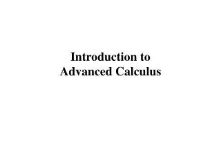
Introduction to Advanced Calculus
1k likes | 1.96k Views
Introduction to Advanced Calculus. (1) In Beginning Calculus , we study functions of one variable. where the input and output are both real numbers. (2) In Intermediate Calculus , we study functions of several variables such as. where the output is still a real number.

Introduction to Advanced Calculus
E N D
Presentation Transcript
(1) In Beginning Calculus, we study functions of one variable where the input and output are both real numbers. (2) In Intermediate Calculus, we study functions of several variables such as where the output is still a real number. (3) In Advanced Calculus, we shall study functions of several variables and with outputs in vectors such as
These are called vector-valued functions, or even Vector Fieldswhen the domain has dimension = dimension of the range, such as Examples: a 2D vector field a surface in 3D a 3D vector field whose z-component is always 0.
A simple case: when the domain is just R and the range is R3, then the function is called a space curve - because each output vector will give a point (namely the endpoint of the vector) in space, and if we joint all these points together, we will get a curve.
Space Curves A space curve is a function C from R to R3, for example note that we do not use the vector notation because we are treating the output as a point in space rather than a vector.
Space curves in 3D In order to see these objects in 3D, you need to have a pair of green-red glasses. The Red lens should be on your left eye, and you may need to dim the surrounding lights to get good results. Even so, it may still take a few seconds for your brain to adjust to the different images seen by different eyes. When you are ready, just click and enjoy.
This is a surface in space. You should be able to determine which part is in the front without the glasses. However the viewing experience in 3D is a lot more satisfying.
1 0 -1 4 2 0 -4 -2 -2 0 2 -4 4 This is a spiral wrapped around a donut. If you move your head sideways slightly, you may see that the curve rotates with you.
1 0.5 0 -0.5 -1 -1.5 -2 -3 -2 -3 -1 -2 0 -1 0 1 1 2 2 3 3 Can you tell which part of the curve is in the front without the glasses?
This is a picture of Mars landscape released by NASA you need to put the red lens on your left eye to see 3D.
Vector Fields in 3D These are functions from R3 to R3 . For any given point P(a,b,c) in space, the arrow initiating from point P represents the output of the function with input (a,b,c).
Smooth Curves and Tangent vector A curve C(t) = (x(t), y(t), z(t)) is smooth in its domain with the functions x(t), y(t), z(t) are all differentiable and throughout the domain. If the curve C(t) is smooth, then the direction of tangent to C(t) at a point t0 is given by the vector The arc length is given by if the curve starts at t = a and ends at t = b.
60 40 20 0 y -4 4 -2 2 0 0 x 2 -2 4 -4 Line Integrals Introduction: Suppose that we have a curve C(t) = ‹ x(t), y(t) › on the xy-plane and a function f(x, y) defined also on the xy-plane. What is the area of the curved surface above the curve and below the surface z = f(x,y)? The red curve isC(t), click to see the surface.
60 40 20 0 y -4 4 -2 2 0 0 x 2 -2 4 -4 Line Integrals Introduction: Suppose that we have a curve C(t) = ‹ x(t), y(t) › on the xy-plane and a function f(x, y) defined also on the xy-plane. What is the area of the curved surface above the curve and below the surface z = f(x,y)? The area is an integral More precise definition will be on the next slide
60 40 20 0 y -4 4 -2 2 0 0 x 2 -2 4 -4 Line Integrals In the following example, f (x, y) = 60 - x2 - y2, and
Line Integrals This type of line integrals can also be defined for function of 3 variables, except that the physical interpretation will no longer be area. Line Integral of a real-valued function Let f(x,y,z) be a real-valued function, and C(t) = (x(t), y(t), z(t)) (for a t b) is a smooth curve in the domain of f , then
More Line Integrals • There are actually two types of line integrals • line integrals of a real-valued function, • line integrals of a vector field. We have already seen the 1st type, and the second type has another physical interpretation. Physical Interpretation If a F is a force field (such as gravity), then the line integral of F along C is the total work done by the force F when a particle moves along the path C. If the integral is positive, then the particle will gain energy (and usually moves faster). Otherwise the particle will slow down. In the special case that the force is always perpendicular to the path, the total work done will be 0.
Line integral of a vector field Let F(x, y, z) = (P(x, y, z), Q(x, y, z), R(x, y, z)) be a vector field and C(t) = (x(t), y(t), z(t)) (for a t b) be a smooth curve in the domain of F, then is called the line integral of F along C.
y 2 1 x -2 -1 1 2 -1 -2 Example
Gradient Vectors fields and the Del Operator Recall that if a function f(x,y,z) from R3 to R has continuous 1st order derivative, then we can derive a vector field which is called the gradient vector field of f. In fact, lots of vector fields are gradient vector fields, and hence we have the following
Gradient Vectors fields and the Del Operator Definition: A vector field F is said to be Conservative if it is the gradient vector field of some differentiable function f(x,y,z), i.e. In this case, f(x,y,z) is called a potential function for F. ( is called the del operator ) Perpetual Machines. http://www.lhup.edu/%7Edsimanek/museum/unwork.htm
Path Independent Integrals Definition A line integral is said to be independent of pathif its value depends only on the end points of the curve C and not on the shape of the curve C (as long as it lies in the domain of F) In other words, if C2 is another path with the same starting and ending points as C, and the trace of C2 also lies in the domain of F, then
Theorem • If F is conservative i.e. F = f for some f , then every line integral of F will be independent of path andwhere (x(a),y(a),z(a)) is the beginning of the curve and (x(b),y(b),z(b)) is the end of the path. • If every line integral of the form is independent of path, then F is conservative.
Corollary F is conservative if and only if for any closed path lying inside the domain of F. We are now going to see several examples of conservative and also non-conservative vector fields.
Examples Dues to the technical difficulties in showing 3D vector fields, we shall only show 2D vector fields.
Is F(x,y) = [x - y, x - 2] conservative? y 4 2 0 -2 -4 x -4 -2 0 2 4
Is F(x,y) = [3 + 2xy, x2 - 3y2] conservative? y 4 2 0 -2 -4 x -4 -2 0 2 4
Is F(x,y) = [2xy + siny, x3 + 2cosy] conservative? y 2 1 0 -1 -2 x -2 -1 0 1 2
Test for Conservativity If F(x, y) = P, Q is a vector field from R2 to R2 with continuous 1st order partial derivatives, then F is conservative if and only if
Definition Given a vector field with differentiable components, we define the divergence of F to be Divergence of a vector field Physical interpretations: If F is the velocity field of some fluid, then F (a,b,c) is the amount of fluid flowing out from the point (a,b,c) in unit time. If F (a,b,c) > 0, then we say that (a,b,c) is a source. If F (a,b,c) < 0, then we say that (a,b,c) is a sink. If F = 0 through out its domain, then we say that F is incompressible.
y 2 1 x -2 -1 1 2 0 -1 -2
Electric field E Gauss Law · E = ρ/εo whereρis chargedensity.
Gauss’s law for Magnetism (2nd of the Maxwell equations) · B = 0 where B stands for magnetic field.
Curl of a vector field Definition Given a vector field F = P, Q, R with differentiable components, we define the Curl of F to be Physical interpretations: If F is the velocity field of some fluid, then × F(a,b,c) is rotation of the fluid at the point (a,b,c), i.e. the magnitude of the vector is the rotational speed and the direction is the direction of rotation according to the right hand rule.
If ×F(a, b, c) = 0,0,0, then we say that F is irrotational at the point (a, b, c). If ×F = 0,0,0 throughout the domain of F, then we say that F is irrotational.
☺ Is the vector field F(x,y,z) = [-y, x, 0] rotational? Conservative? y 4 2 x -4 -2 2 4 0 -2 -4
☺ Is the vector field F(x,y,z) = [x + y, x – y, 0] rotational? Is it Compressible? y 4 2 x 0 -4 -2 2 4 -2 -4
Test for Conservativity Theorem If f(x,y,z) is a function from R3 to R which has continuous 1st order partial derivatives, then Curl(f) = ×f = 0,0,0 If F(x, y, z) = P, Q, R is a vector field from R3 to R3 with continuous 1st order partial derivatives, then F is conservative if and only if CurlF = ×F = 0,0,0 As a consequence, we see that F is conservative if and only if it is irrotational.
The following vector field is clearly rotational (at many points), hence not conservative. y 4 2 x -4 -2 0 2 4 -2 -4
Clay Mathematics Institute • Millennium Problems • In order to celebrate mathematics in the new millennium, The Clay Mathematics Institute of Cambridge, Massachusetts (CMI) has named seven Prize Problems. The Scientific Advisory Board of CMI selected these problems, focusing on important classic questions that have resisted solution over the years. The Board of Directors of CMI designated a $7 million prize fund for the solution to these problems, with $1 million allocated to each. • One hundred years earlier, on August 8, 1900, David Hilbert delivered his famous lecture about open mathematical problems at the second International Congress of Mathematicians in Paris. This influenced our decision to announce the millennium problems as the central theme of a Paris meeting. • Paris, May 24, 2000 • Birch and Swinnerton-Dyer Conjecture • Hodge Conjecture • Navier-Stokes Equations • P vs NP • Poincaré Conjecture • Riemann Hypothesis • Yang-Mills Theory
Navier-Stokes Equation Waves follow our boat as we meander across the lake, and turbulent air currents follow our flight in a modern jet. Mathematicians and physicists believe that an explanation for and the prediction of both the breeze and the turbulence can be found through an understanding of solutions to the Navier-Stokes equations. Although these equations were written down in the 19th Century, our understanding of them remains minimal. The challenge is to make substantial progress toward a mathematical theory which will unlock the secrets hidden in the Navier-Stokes equations.