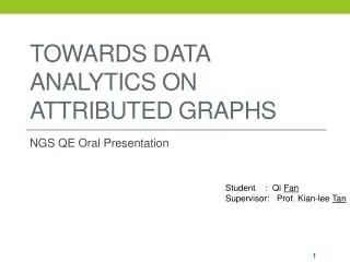
Towards Data Analytics on Attributed Graphs

1. Towards Data Analytics on Attributed Graphs NGS QE Oral Presentation Student : Qi Fan Supervisor: Prof. Kian-lee Tan

2. Outline Attributed Graph Analytic Graph Window Query Graph Window Query Processing Experiments Future Works

3. Outline • Attributed Graph Analytic • Graph Window Query • Graph Window Query Processing • Experiments • Future Works

4. Data Analytics [1] Analytics Examples: http://en.wikipedia.org/wiki/Analytics • Data Analytics plays an important part in business [1] • Web analytics for advertising and recommendation • Customer analytics for market optimization • Portfolio analytics for risk control • Analytics on data yield: • Data products • Data-driven decision support • Insights of data model

5. Relational Data Analytic • Table as data representation, SQL as the query language • Analytic SQL: • Ranking • Windowing • LAG/LEAD • FIRST/LAST • SKYLINE • TOP-K • … …

6. Emerging of Large Linked Data [1] http://java.dzone.com/articles/mysql-vs-neo4j-large-scale • In real world, linked data are becoming emerging: • Facebook, LinkedIn, Biological network, Phone Call network, Twitter, etc. • Modeling linked data in relational way and querying using SQL is inefficient: • Graph queries are often traverse based • SQL based traversal is 100 times slower than adjacent list based [1] • Graph model is more fit for linked data!!!

7. Graph Data Model Vertex Edge G = (V, E, A) Attributed Graph Vertices Edges Attributes Graph Attribute Table Graph Structure +attribute dimensions

8. Graph Data Model • Graph Data: • Vertex – entities, i.e. User, Webpage, Molecule, etc. • Edge – relationships, i.e. follow, cite, depends-on, friends-of, etc. • Attribute – profile information for vertex/edge • Specific model depends on data, thus: • Edge – directed / undirected • Attribute – homogeneous, inhomogeneous

9. Graph Data Model Example People and friends relationships… People and follow relationships... Attributed Graph modelsa wealth of information Bimolecules and depends-on relationships...

10. Graph Data Analytics [1] Tian, Y., Hankins, R. A., & Patel, J. M. (2008, June). Efficient aggregation for graph summarization. In Proceedings of the 2008 ACM SIGMOD • Graph Database environment is growing: • Neo4j, Titan, SPARQL, Pregel etc. • Graph Data Analytics are becoming popular: • Graph Summarization[1], Graph OLAP [2] etc. • In our research, we focus on: • Discover needs of native graph analytical queries • Process graph analytical query efficiently [2] C. Chen, X. Yan, F. Zhu, J. Han, and P. S. Yu, “Graph olap: Towards online analytical processing on graphs,” in Data Mining, 2008. ICDM’08

11. Outline • Attributed Graph Analytic • Graph Window Query • Graph Window Query Processing • Experiments • Future Works

12. SQL Window Query Window of a tuple contains other tuples relatedto it Window of Tuple 7 • A SQL window query: • Partitions a table • Sorts each partition • Implicitly forms window of each tuple

13. Graph Window Query In graph, a vertex can also have a set of relatedvertices to be its window. The aggregation on window is a personalizedanalysisover each vertex.

14. Graph Window Examples Summarizing the age distribution of eachuser’s friends Summarizing the activeness of eachuser’s friends Analyze the industry distribution of a user potential connections These queries focus on the neighborhoods of each user, thus the neighborhoodsforms a vertex’s window

15. Graph Window Examples Find how many enzymes are in eachmolecule’s pathway Find how many molecules are affected by each enzymein the pathway These queries focus on the ancestor-descendent relationship of molecules, thus ancestor-descendent is a vertex’s window

16. Graph Window Queries • We thus identify two types of graph window queries: • K-hop window (k-window): • A vertex’s k-hop window contains all the vertices that are its the k-hopneighbors. • Topological window (t-window): • A vertex’s topological window contains all the vertices that are its accentors / descendents

17. Graph Window Queries • K-hop Window: • Similar to ego-centric analysis of network analysis community • For undirected graph: • all vertices that can connect a vertex • For directed graph: • In-k-hop, for vertices that reaches a vertex in k-hop • Out-k-hop, for vertices that reached by a vertex in k-hop • K-hop, union of in-k-hop and out-k-hop • T-Window: • Requires graph to be DAG

18. Graph Window Queries • Graph Window Query: • INPUT: a specific window (k-hop, topological) and an aggregation function • OUTPUT: aggregated value over each vertex’s window

19. Outline • Attributed Graph Analytic • Graph Window Query • Graph Window Query Processing • Experiments • Future Works

20. Related Work [1] J. Mondal and A. Deshpande, “Eagr: Supporting continuous ego-centric aggregate queries over large dynamic graphs,” SIGMOD, 2015. • In [1] a system EAGr has been proposed to process neighborhood query • Focuses on 1-hop neighbor • It uses iterative planning methods to share aggregations results between different vertex’s window • However, it assumes a large intermediate data to reside in memory, which is not reasonable for k-window () and t-window

21. Graph Window Query Processing • Naïve Processing I: • Compute vertex’s window sequentially • Aggregate each vertex individually • Advantage: • No large intermediate data generated • Inefficiencies: • Repeated computation of every vertex’s window: • k-window is of complexity in arbitrary graph • t-window is of complexity in arbitrary graph • Slow in individual aggregation: • Each vertex may have window size of • Total aggregation complexity can be

22. Graph Window Query Processing • Naïve Processing II: • Materialize each vertex’s window • On query processing, aggregate each vertex’s window individually • Advantage: • No computation of windows at run time • Inefficiencies: • Materialize is not memory efficient • All the vertex’s window can be as large as • Query processing is still slow as in Naïve Processing I

23. Overview of our approach • Two index schemes: • Dense Block Index: for general window and k-hop window • Parent Index: for topological window • Indexes achieves: • Completely preserve the window information for each vertex • Space efficiency • Efficient run-time query processing

24. Dense Block Index – Matrix View • Window Matrix: • Records vertex-window mapping • Rows represent vertex • Columns represent window

25. Dense Block Index – Matrix View • Window Matrix Properties: • Boolean matrix • Completely keeps the vertex-window information • Equivalent Matrices: • Window matrix can be applied with row and column permutations • Invariant: number of non-zero elements ()

26. Dense Block Index – Matrix View • Window matrix based aggregation: • Similar to Naïve Processing II • Traverse the matrix vertically • Aggregate the cells with value one, ignore cells with value zero • Space and Query Complexity: • in sparse matrix format • in matrix format • Note that can be as large as

27. Dense Block Index Same asymptotical bounds, thus can optimize both simultaneously Store row id and column id i.e. (A,B)(A,B,C) rather than 6 elements Query: Compute A+B first, then the result is shared for window (A,B,C) • Dense Blocks: • Given a matrix, dense blocks is the submatrix whose values are all non-zeros • Properties of Dense Blocks (): • Space complexity • compared to • Query complexity • compared to

28. Dense Block Index • Dense Block Index: • For every window to be computed, index all the dense blocks in a window matrix • A bipartite graph

29. Dense Block Index • Properties: • Preserves every non-zero entry of window matrix • During query, no need to access original window matrix • Query Processing: • compute partial aggregates for each dense block • compute final aggregates for every window

30. Dense Block Index Query Processing Compute OnGraph G Over 1-hop Window Summarizing the activeness of each user’s friends:

31. Dense Block Index [1] V. Vassilevska and A. Pinar, “Finding nonoverlapping dense blocks of a sparse matrix,” Lawrence Berkeley National Laboratory, 2004 • Equivalent matrices may have different optimal partitions • Find best dense block partition out of all equivalent matrices • Fixed size dense block partition is NP-hard [1] • Heuristics need to be applied

32. MinHash Clustering for DBI • Heuristic • Classifies similar windows together, then mining the dense blocks in each cluster • Clustering + Mining • Clustering: • Jaccard coefficient is used to measure the similarity between windows • Since each window is a set of vertices • MinHash is an efficient way to perform Jaccard coefficient based clustering

33. MinHash Clustering for DBI • Mining: • Build partial window matrix for each cluster • Condense the rows with identical values • For uncondensed rows, recursively cluster + mining, until stop condition achieves

34. MinHash Clustering for DBI MinHash Clustering Recursive cluster Outputs Outputs Split

35. MinHash Clustering for DBI Bottlenecks MINHASH COST: WINDOW COST: for k-window, for t-window Too HIGH in practice • DBI generation can be summarized into following steps: • Clustering Step: • Min-Hash each vertex, based on its window • Mining Step: • Generate partial matrix for each window • Group identical rows • Recursive clustering

36. Estimated MinHash Clustering • For K-hop, we developed an estimation scheme to speed up the index creation process. • The observation is that when hop goes larger, the overlapping between each vertex also goes larger • Thus we can use lower hop window information in the clustering phase

37. Comparison • MinHash Clustering • Clustering Step: • Min-Hash each vertex, based on its window • Mining Step: • Generate partial matrix for each window • Group Identical rows • Recursive clustering • Estimated Clustering • Clustering Step: • Min-Hash each vertex, based on its lower-hop window • Mining Step: • Generate partial matrix for each window • Group Identical rows • Recursive clustering The estimation reduces the indexing time since: Lower-hop window has less elements, so MinHash is faster Lower-hop window generation requires less time

38. Topological Window Processing • Dense Block Index can be used on Topological Window as well • However, more efficient index exists given a T-window query • Containment Relationship in T-window • If , then • Thus, when compute window of , ’s result can be directly used.

39. Parent Index Given , in order to use for computing , we need to materialize the difference between and For a given , the vertex with smallest difference must be one of ’s parent Thus, for each vertex, we only index its parent which has the smallest different

40. Parent Index • A parent index is a lookup table of three fields: • Vertex: the index entry • Parent: the closest parent id • Diff: the difference vertices between Vertexand Parent

41. Parent Index based Query Processing • Topologically process each vertex’ window • Use the formulae: • Topological order ensures that when processing a vertex, its parents’ results are ready

42. Parent Index Creation • Efficiently creation based on Topological Scan: • During scan, each vertex passes its current ancestor information to its child • Child on receiving parents’ ancestor information, union these ancestors • Child on receiving all parents information, record the portent with smallest difference

43. Outline • Attributed Graph Analytic • Graph Window Query • Graph Window Query Processing • Experiments • Future Works

44. Experiments [1] Stanford Networ Analysis Platform, http://snap.stanford.edu/snap/index.html [2] H. Yildirim, V. Chaoji, and M. J. Zaki, “Dagger: A scalable index for reachability queries in large dynamic graphs,” arXiv preprint arXiv:1301.0977, 2013. • Machine: 2.27GHz CPU with 32 GB memory • Data Synthetic: • SNAP [1] generator for directed graphs • DAGGR [2] generator for DAGs

45. Comparing Algorithms • K-hop window: • MA: materialize ahead algorithm (materialize vertex-window mapping, individual aggregate) • KBBFS: bounded BFS for computing window of each vertex • MC: MinHash Clustering • EMC: Estimated MinHash Clustering • Topological window: • MA • DBI: dense block index • TS: Topological Scan to compute window of each vertex • PI: parent index

46. Effectiveness of Estimation Hop = 1 Hop = 2 Hop = 4 Hop = 3

47. Benefit of Estimation Degree 160 Degree 40

48. Index size of MC and EMC Degree = 40

49. Scalability of EMC V = 100k, hop =1 V = 100k, hop = 2

50. Effectiveness of PI V = 10k