Download
1 / 75
750 likes | 887 Views
CSE 634 Data Mining Techniques. CLUSTERING Part 2( Group no: 1 ) By: Anushree Shibani Shivaprakash & Fatima Zarinni Spring 2006 Professor Anita Wasilewska SUNY Stony Brook. References. Jiawei Han and Michelle Kamber. Data Mining Concept and Techniques (Chapter8) . Morgan Kaufman, 2002.

E N D
CSE 634 Data MiningTechniques CLUSTERING Part 2( Group no: 1 ) By: Anushree Shibani Shivaprakash & Fatima Zarinni Spring 2006 Professor Anita WasilewskaSUNY Stony Brook
References • Jiawei Han and Michelle Kamber. Data Mining Concept and Techniques (Chapter8). Morgan Kaufman, 2002. • M. Ester, H.P. Kriegel, J. Sander, and X. Xu. A density-based algorithm for discovering clusters in large spatial databases. KDD'96. http://ifsc.ualr.edu/xwxu/publications/kdd-96.pdf • How to explain hierarchical clustering. http://www.analytictech.com/networks/hiclus.htm • Tian Zhang, Raghu Ramakrishnan, Miron Livny. Birch: An efficient data clustering method for very large databases • Data mining- Margaret H. Dunham • http://cs.sunysb.edu/~cse634/ Presentation 9 – Cluster Analysis
Introduction Major clustering methods • Partitioning methods • Hierarchical methods • Density-based methods • Grid-based methods
Hierarchical methods • Here we group data objects into a tree of clusters. • There are two types of hierarchical clustering • Agglomerative hierarchical clustering. • Divisive hierarchical clustering
Agglomerative hierarchical clustering • Group data objects in a bottom-up fashion. • Initially each data object is in its own cluster. • Then we merge these atomic clusters into larger and larger clusters, until all of the objects are in a single cluster or until certain termination conditions are satisfied. • A user can specify the desired number of clusters as a termination condition.
Divisive hierarchical clustering • Groups data objects in a top-down fashion. • Initially all data objects are in one cluster. • We then subdivide the cluster into smaller and smaller clusters, until each object forms cluster on its own or satisfies certain termination conditions, such as a desired number of clusters is obtained.
Step 0 Step 1 Step 2 Step 3 Step 4 agglomerative (AGNES) a a b b a b c d e c c d e d d e e divisive (DIANA) Step 3 Step 2 Step 1 Step 0 Step 4 AGNES & DIANA • Application of AGNES( AGglomerative NESting) and DIANA( Divisive ANAlysis) to a data set of five objects, {a, b, c, d, e}.
AGNES-Explored • Given a set of N items to be clustered, and an NxN distance (or similarity) matrix, the basic process of Johnson's (1967) hierarchical clustering is this: • Start by assigning each item to its own cluster, so that if you have N items, you now have N clusters, each containing just one item. Let the distances (similarities) between the clusters equal the distances (similarities) between the items they contain. • Find the closest (most similar) pair of clusters and merge them into a single cluster, so that now you have one less cluster.
AGNES • Compute distances (similarities) between the new cluster and each of the old clusters. • Repeat steps 2 and 3 until all items are clustered into a single cluster of size N. • Step 3 can be done in different ways, which is what distinguishes single-link from complete-link and average-link clustering
Similarity/Distance metrics • single-link clustering, distance = shortest distance • complete-link clustering, distance =longest distance • average-link clustering, distance = average distance from any member of one cluster to any member of the other cluster.
Single Linkage Hierarchical Clustering • Say “Every point is its own cluster”
Single Linkage Hierarchical Clustering • Say “Every point is its own cluster” • Find “most similar” pair of clusters
Single Linkage Hierarchical Clustering • Say “Every point is its own cluster” • Find “most similar” pair of clusters • Merge it into a parent cluster
Single Linkage Hierarchical Clustering • Say “Every point is its own cluster” • Find “most similar” pair of clusters • Merge it into a parent cluster • Repeat
Single Linkage Hierarchical Clustering • Say “Every point is its own cluster” • Find “most similar” pair of clusters • Merge it into a parent cluster • Repeat
DIANA (Divisive Analysis) • Introduced in Kaufmann and Rousseeuw (1990) • Inverse order of AGNES • Eventually each node forms a cluster on its own
Overview • Divisive Clustering starts by placing all objects into a single group. Before we start the procedure, we need to decide on a threshold distance. The procedure is as follows: • The distance between all pairs of objects within the same group is determined and the pair with the largest distance is selected.
Overview-contd • This maximum distance is compared to the threshold distance. • If it is larger than the threshold, this group is divided in two. This is done by placing the selected pair into different groups and using them as seed points. All other objects in this group are examined, and are placed into the new group with the closest seed point. The procedure then returns to Step 1. • If the distance between the selected objects is less than the threshold, the divisive clustering stops. • To run a divisive clustering, you simply need to decide upon a method of measuring the distance between two objects.
DIANA- Explored • In DIANA, a divisive hierarchical clustering method, all of the objects form one cluster. • The cluster is split according to some principle, such as the minimum Euclidean distance between the closest neighboring objects in the cluster. • The cluster splitting process repeats until, eventually, each new cluster contains a single object or a termination condition is met.
Difficulties with Hierarchical clustering • It encounters difficulties regarding the selection of merge and split points. • Such a decision is critical because once a group of objects is merged or split, the process at the next step will operate on the newly generated clusters. • It will not undo what was done previously. • Thus, split or merge decisions, if not well chosen at some step, may lead to low-quality clusters.
One promising direction for improving the clustering quality of hierarchical methods is to integrate hierarchical clustering with other clustering techniques. A few such methods are: Birch Cure Chameleon Solution to improve Hierarchical clustering
BIRCH: An Efficient Data Clustering Method for Very Large Databases Paper by: Miron Livny Computer Sciences Dept. University of Wisconsin- Madison miron@cs.wisc.edu Raghu Ramakrishnan Computer Sciences Dept. University of Wisconsin- Madison raghu@cs.wisc.edu Tian Zhang Computer Sciences Dept. University of Wisconsin- Madison zhang@cs.wisc.edu In Proceedings of the International Conference Management of Data (ACM-SIGMOD), pages 103-114, Montreal, Canada, June, 1996.
Reference For Paper • www2.informatik.huberlin.de/wm/mldm2004/zhang96birch.pdf
Birch (Balanced Iterative Reducing and Clustering Using Hierarchies) • A hierarchical clustering method. • It introduces two concepts : • Clustering feature • Clustering feature tree (CF tree) These structures help the clustering method achieve good speed and scalability in large databases.
Clustering Feature Definition Given N d-dimensional data points in a cluster: {Xi} where i = 1, 2, …, N, CF = (N, LS, SS) N is the number of data points in the cluster, LS is the linear sum of the N data points, SS is the square sum of the N data points.
Clustering feature concepts • Each record (data object) is a tuple of values of attributes and here is called a vector. Here is a database. We define (Vi1, …Vid) = Oi N N N N LS = ∑ Oi = (∑Vi1, ∑ Vi2,… ∑Vid) i=1 i=1 i=1 i =1 Linear Sum Definition Definition Name
Square sum NN N N SS = ∑ Oi2 = ( ∑Vi12, ∑Vi22… ∑Vid2) i =1 i=1 i=1 i=1 Definition Name
Example of a case Assume N = 5 and d = 2 Linear Sum 5 5 5 LS = ∑ Oi = (∑Vi1, ∑ Vi2) i=1 i=1 i=1 Square Sum 5 5 SS =( ∑Vi12), ∑Vi22) i=1 i=1
Example 2 Clustering feature = CF=( N, LS, SS) N = 5 LS = (16, 30) SS = ( 54, 190) CF = (5, (16,30),(54,190))
CF-Tree • A CF-tree is a height-balanced tree with two parameters: branching factor (B for nonleaf node and L for leaf node) and threshold T. • The entry in each nonleaf node has the form [CFi, childi] • The entry in each leaf node is a CF; each leaf node has two pointers: `prev' and`next'. • The CF tree is basically a tree used to store all the clustering features.
CF1 CF2 CF3 CF6 child1 child2 child3 child6 CF Tree Root Non-leaf node CF1 CF2 CF3 CF5 child1 child2 child3 child5 Leaf node Leaf node prev CF1 CF2 CF6 next prev CF1 CF2 CF4 next
BIRCH Clustering • Phase 1: scan DB to build an initial in-memory CF tree (a multi-level compression of the data that tries to preserve the inherent clustering structure of the data) • Phase 2: use an arbitrary clustering algorithm to cluster the leaf nodes of the CF-tree
Summary of Birch • Scales linearly- with a single scan you get good clustering and the quality of clustering improves with a few additional scans. • It handles noise (data points that are not part of the underlying pattern) effectively.
Density-Based Clustering Methods • Clustering based on density, such as density-connected points instead of distance metric. • Cluster = set of “density connected” points. • Major features: • Discover clusters of arbitrary shape • Handle noise • Need “density parameters” as termination condition- (when no new objects can be added to the cluster.) • Example: • DBSCAN (Ester, et al. 1996) • OPTICS (Ankerst, et al 1999) • DENCLUE (Hinneburg & D. Keim 1998)
p MinPts = 5 Eps = 1 q Density-Based Clustering: Background • Eps neighborhood: The neighborhood within a radius Eps of a given object • MinPts: Minimum number of points in an Eps-neighborhood of that object. • Core object :If the Eps neighborhood contains at least a minimum number of points Minpts, then the object is a core object • Directly density-reachable: A point p is directly density-reachable from a point q wrt. Eps, MinPts if 1) p is within the Eps neighborhood of q 2) q is a core object
Figure showing the density reachability and density connectivity in density based clustering • M, P, O, R and S are core objects since each is in an Eps neighborhood containing at least 3 points Minpts = 3 Eps=radius of the circles
Directly density reachable Q is directly density reachable from M. M is directly density reachable from P and vice versa.
Indirectly density reachable • Q is indirectly density reachable from P since Q is directly density reachable from M and M is directly density reachable from P. But, P is not density reachable from Q since Q is not a core object.
Core, border, and noise points • DBSCAN is a density-based algorithm. • Density = number of points within a specified radius (Eps) • A point is a core point if it has more than a specified number of points (MinPts) within Eps • These are points that are at the interior of a cluster. • A border point has fewer than MinPts within Eps, but is in the neighborhood of a core point. • A noise point is any point that is not a core point nor a border point.
DBSCAN (Density based Spatial clustering of Application with noise): The Algorithm • Arbitrary select a point p • Retrieve all points density-reachable from p wrt Eps and MinPts. • If p is a core point, a cluster is formed. • If p is a border point, no points are density-reachable from p and DBSCAN visits the next point of the database. • Continue the process until all of the points have been processed.
Conclusions • We discussed two hierarchical clustering methods – Agglomerative and Divisive. • We also discussed Birch- a hierarchical clustering which produces good clustering over a single scan and with a few additional scans you get better clustering. • DBSCAN is a density based clustering algorithm and through this algorithm we discover clusters of arbitrary shapes. Distance is not the metric unlike the case of hierarchical methods.
GRID-BASED CLUSTERING METHODS • This is the approach in which we quantize space into a finite number of cells that form a grid structure on which all of the operations for clustering is performed. • So, for example assume that we have a set of records and we want to cluster with respect to two attributes, then, we divide the related space (plane), into a grid structure and then we find the clusters.
Salary (10,000) Our “space” is this plane 8 7 6 5 4 3 2 1 0 20 30 40 50 60 Age
Techniques for Grid-Based Clustering The following are some techniques that are used to perform Grid-Based Clustering: • CLIQUE (CLustering In QUest.) • STING (STatistical Information Grid.) • WaveCluster
Looking at CLIQUE as an Example • CLIQUE is used for the clustering of high-dimensional data present in large tables. By high-dimensional data we mean records that have many attributes. • CLIQUE identifies the dense units in the subspaces of high dimensional data space, and uses these subspaces to provide more efficient clustering.
Definitions That Need to Be Known • Unit :After forming a grid structure on the space, each rectangular cell is called a Unit. • Dense:A unit is dense, if the fraction of total data points contained in the unit exceeds the input model parameter. • Cluster:A cluster is defined as a maximal set of connected dense units.
How Does CLIQUE Work? • Let us say that we have a set of records that we would like to cluster in terms of n-attributes. • So, we are dealing with an n-dimensional space. • MAJOR STEPS : • CLIQUE partitions each subspace that has dimension 1 into the same number of equal length intervals. • Using this as basis, it partitions the n-dimensional data space into non-overlapping rectangular units.
CLIQUE: Major Steps (Cont.) • Now CLIQUE’S goal is to identify the dense n-dimensional units. • It does this in the following way: • CLIQUE finds dense units of higher dimensionality by finding the dense units in the subspaces. • So, for example if we are dealing with a 3-dimensional space, CLIQUE finds the dense units in the 3 related PLANES (2-dimensional subspaces.) • It then intersects the extension of the subspaces representing the dense units to form a candidate search space in which dense units of higher dimensionality would exist.
CLIQUE: Major Steps. (Cont.) • Eachmaximal set of connected dense units is considered a cluster. • Using this definition, the dense units in the subspaces are examined in order to find clusters in the subspaces. • The information of the subspaces is then used to find clusters in the n-dimensional space. • It must be noted that all cluster boundaries are either horizontal or vertical. This is due to the nature of the rectangular grid cells.