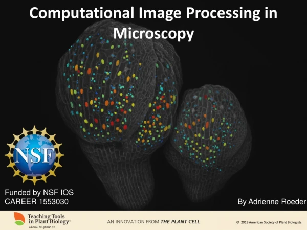
Computational Image Processing in Microscopy
Learn about computational image analysis, microscopy image processing, fluorescence microscopy, and confocal microscopy techniques in this informative workshop. Understand image processing pipelines and considerations for acquiring microscopy images.


Computational Image Processing in Microscopy
E N D
Presentation Transcript
Computational Image Processing in Microscopy Funded by NSF IOS CAREER 1553030 By Adrienne Roeder
Learning objectives • Develop the vocabulary to communicate about computational image analysis. • Identify properties of images that make them amenable to computational image analysis. • Understand how microscopy images are generated. • Discuss the advantages and limitations of various image analysis tools. • Distinguish between unacceptable image manipulation and quantitative image analysis. • Apply the COSTANZA image analysis tool in Fiji to analyze research images (Workshop).
Part 1. Image processing • Uses computational algorithms, sometimes with manual intervention, to extract information (features, measurements, patterns, etc.) from digital images. • Allows extraction of quantitative data from large image datasets. Image processing Developing Arabidopsis flower expressing mCitrine-ATML1 fluorescent transcription factor fusion protein Processed image detecting each sepal nucleus and quantifying mCitrine-ATML1 fluorescence Meyer HM, Teles J, Formosa-Jordan P, et al. Fluctuations of the transcription factor ATML1 generate the pattern of giant cells in the Arabidopsis sepal. eLife. 2017;6:e19131. doi:10.7554/eLife.19131.
Typical image processing pipeline Microscopy Original image Pre-processing Segmentation Post-processing Data analysis
Step 1: Imaging Microscopy Original image Pre-processing Segmentation Post-processing Data analysis
Considerations in acquiring a microscopy image for computational processing • Simple images with the objects in one color and the background in black work best. • The structure of interest should be one color and nothing else the same color. • There should be high contrast between objects of interest and background. • Microscope settings should be adjusted to take images optimized for computational processing, not viewing. Difficult for image processing: poor contrast, multiple features in the same color range Good for image processing: split colors
Standard light microscopy (bright field) camera Eyepiece • Light microscopes use visible light and magnifying lenses to visualize samples. • Standard light microscopes must make light transmit through the sample, which often requires clearing or sectioning. • Stains can be used to add contrast and can be specific to certain features. • Images tend to be difficult for analysis by image processing due to the complexity of colors and shadings. Lenses Focus Knobs stage condenser Toluidine blue stain Cross section of Arabidopsis fruit bulb mirror
Fluorescence microscopy • Advantage: great specificity. You only see fluorophores (usually fluorescent proteins or dyes you added to the sample) that you have excited with the light you shine on them good for image processing • Advantage: sample can be alive! • Limitations: bleaching, auto-fluorescence, bleed-through of one color channel into another. 48 h Fluorescence image (confocal) of an Arabidopsis seedling Living, developing Arabidopsis flower bud (confocal)
Fluorescence Excited state Excitation and emission spectra of GFP 100% excitation 80% emission Absorption of blue photon Emission of green photon 60% Normalized fluorescence 40% Ground state 20% 0% 300 350 400 450 500 550 600 GFP emission detected Wavelength (nm) 488 laser excitation • Shorter wavelength = more energy. • A fluorophore (e.g., Green Fluorescent Protein GFP) absorbs light of a shorter wavelength (e.g., blue), exciting the fluorophore, and emits light at a longer wavelength (e.g. green). • Each fluorophore has a a characteristic excitation and emission spectrum.
Fluorescence microscopy light path camera eyepiece Dichroic mirrors reflect light at some wavelengths (excitation) and let light at other wavelengths (emission) pass through. emisssion dichroic mirror excitation lenses focus Knobs stage condenser • Excitation light from a light source hits a dichroic mirror and is reflected down through the objective lens to the specimen. It excites the fluorophores in the specimen, which emit a longer wavelength emission light. The emission light enters the objective, passes through the dichroic mirror and other filters to be recorded by the camera.
detector Confocal microscopy uses a pinhole to optically section the sample detector pinhole out of focal plane light blocked laser dichroic mirror excitation emisssion in focal plane light detected light source pinhole detector lenses Sunflower pollen grain pinhole focus Knobs stage Widefield Confocal condenser Objective lens Focal plane https://www.olympus-lifescience.com/en/microscope-resource/primer/techniques/confocal/confocalintro/ • Pinholes create optical sections – light from outside the focal plane is blocked by the pinhole (diffuse green). Only in-focus light rays initiated in the focal plane pass through the pinhole (green line) to the detector. Image source: Olympus
detector Confocal microscopy images are generated by laser scanning detector pinhole laser dichroic mirror excitation eyepiece emisssion Laser illuminates one point Laser illuminates the next point Intensity = 59 Light source pinhole Intensity = 129 lenses focus Knobs stage condenser Diagram of a typical scanning pattern of the laser across the sample to capture the whole optical section. • The laser is used to excite the fluorophores at one point in the sample. • The detector (often a photomultiplier tube or PMT) quantitatively detects the amount of emission light from that point in the sample and records it as a pixel in the image. • Then the laser moves over to collect data at the next point.
Different fluorophores can be recorded in separate channels • Samples often have 2 or more fluorophores, which are spectrally distinct (e.g., GFP and chlorophyll). • Each fluorophore can be recorded in a separate channel using different excitation and/or emission wavelengths. • Different detectors can be used to simultaneously record each fluorophore or the same detector can be used sequentially. • Each channel can be displayed in a different color in the composite image. • Consider color blindness in the choice of colors (i.e., not green/red) Channel 1: nuclei Channel 2: chlorophyll Composite Excitation 488 Emission 493-556 Excitation 488 Emission 593-710 Channel 1: green Channel 2: magenta Colors assigned by user
“Z-stack” captures the 3D image • 3D image composed of a series 2D optical section images collected from a single biological sample. Z-stack Microscope control
Pixel and voxel • Pixels and voxels are the basic units of the image. • Each has an associated intensity value measured by the detector (from 0 for black to 255 for white in an 8 bit image). • Each represents a defined unit of area or volume in the sample, which is recorded in the microscope metadata. • A voxel is the 3D analog to the pixel. Pixel: 2D Voxel: 3D Green intensity value of each pixel Green intensity value of each voxel 8 46 65 208 45 142 1 voxel represents 0.755 µm × 0.755 µm × 4.0 µm 24 70 149 1 pixel represents 0.755 µm × 0.755 µm
Resolution and dots per inch • Resolution is the ability to resolve or distinguish features in the image. • The resolution is limited by intrinsic properties of the imaging system. • Printing resolution is the number of dots (pixels) per unit distance, e.g. dots per inch (DPI). • Journals generally require 300 DPI for images. • Resampling to decrease pixels is acceptable, resampling to increase pixels is not acceptable. 1024 x 1024 image 600 DPI 1024 x 1024 image 300 DPI
Limits of resolution of light microscopy surpassed with super-resolution • Two individual fluorophores that are closer together than the diffraction limit of the microscope, which depends on the wavelength of light, cannot be resolved with traditional microscopy (e.g., 2 GFP proteins < 500 nm apart). • A number of different super-resolution techniques have recently been developed to overcome this barrier. Super-resolution Structured illumination (SIM) Widefield fluorescence Confocal Cortical microtubules in the hypocotyl George Komis, G. et al. (2014). Dynamics and organization of cortical microtubules as revealed by superresolution structured ilumination microscopy. Plant Physiol. 165: 129-148.
Maximum intensity projection • For each pixel in the image, the algorithm selects the brightest slice from the z-stack. These brightest pixels are combined to make the final image. • The maximum intensity projection often can be used to produce an overall view of the specimen, particularly the outer surface.
Image Compression • Reduces the size of the image file by filtering redundant information. • Lossless compression: The exact image can be recovered, e.g., LZW in TIFF. • Lossy compression: Information is lost, e.g., JPEG. Original image Highly compressed lossy Roeder AHK, Cunha A, Burl MC, Meyerowitz EM. (2012) A computational image analysis glossary for biologists. Development 139: 3071-3080. doi:10.1242/dev.076414.
Step 2: Pre-processing Microscopy Original image Pre-processing Segmentation Post-processing Data analysis
Denoising filters • Denoising filters compare a targetpixel to the surrounding pixels and change the intensity value of the target pixel based on the neighbor values. • Mean = mean of neighbors; median = median of neighbors; Gaussian blur = the weighted average of the pixel and its neighbors, with the weight assigned according to distance. median Gaussian blur original mean
Step 3: Segmentation Microscopy Original image Pre-processing Segmentation Post-processing Data analysis
Segmentation • Segmentation automatically delineates objects in the image for further analysis. • Segmentation is the process of partitioning an image into regions of interest, i.e., identifying each nucleus, cell, or tissue type within the image.
Thresholding segmentation • Thresholding is a simple method of segmentation. The user defines a threshold intensity and everything above it is marked as objects and everything below it is marked as background. • It is used in COSTANZA as a pre-processing step (Background Extraction). • It does not work well when different objects have different intensity. • Fiji: Image>Adjust>Threshold Roeder AHK, Cunha A, Burl MC, Meyerowitz EM. (2012) A computational image analysis glossary for biologists. Development 139: 3071-3080. doi:10.1242/dev.076414.
Gradient ascent/descent segmentation • A segmentation method for finding local image intensity maxima/minima (e.g., the center of the nucleus). • An image can be thought of as landscape with peaks and valleys in intensity. • The algorithm starts from each pixel in the image, moves to the neighboring pixel with the highest intensity and repeats the process, until no neighbor has a higher intensity. This is the local maximum. • Good for identifying objects that do not have the same intensity. • BOA = Basin of attraction = all the points that associate with the same maximum intensity COSTANZA uses gradient ascent
Watershed segmentation Fills each cell like water poured into the intensity landscape. Seed each cell Watershed segmentation of tomato shoot apex cells in MorphoGraphX software. Barbier de Reuille P, Routier-Kierzkowska AL, Kierzkowski D, et al. MorphoGraphX: A platform for quantifying morphogenesis in 4D. eLife. 2015;4:e05864. doi:10.7554/eLife.05864.001.
Edge detection segmentation • Finds edges of objects by detecting steep changes in image intensity. • Fiji: Process>Find edges • Plugin Canny edge detection (https://imagej.nih.gov/ij/plugins/canny/index.html) original edge detect Roeder AHK, Cunha A, Burl MC, Meyerowitz EM. (2012) A computational image analysis glossary for biologists. Development 139: 3071-3080. doi:10.1242/dev.076414.
Step 4: Post-processing Microscopy Original image Pre-processing Segmentation Post-processing Data analysis
Semi-automated approach • Automated segmentation programs commonly make errors that are obvious to the scientist. • Scientists often correct errors generated by the automated segmentation program by hand. • Critique: can add human bias. Hand correction Added Erased Automated segmentation Final segmentation Original image Some errors Roeder AHK, Cunha A, Burl MC, Meyerowitz EM. (2012) A computational image analysis glossary for biologists. Development 139: 3071-3080. doi:10.1242/dev.076414.
Registration • Alignment of two images. • Often used to compare time points. Live imaging of nuclei in developing Arabidopsis flowers 0 hours 6 hours Roeder AHK, Cunha A, Burl MC, Meyerowitz EM. (2012) A computational image analysis glossary for biologists. Development 139: 3071-3080. doi:10.1242/dev.076414.
Tracking • Identifying corresponding features (i.e. nuclei, cells, etc.) in images from a time series. Roeder AHK, Cunha A, Burl MC, Meyerowitz EM. (2012) A computational image analysis glossary for biologists. Development 139: 3071-3080. doi:10.1242/dev.076414.
Validation Processed image Original • Carefully compare results with original image.
Summary of Image Processing • Computational image processing provides a powerful tool to extract quantitative information from a large image dataset. • During image acquisition, images should be optimized for future processing. Confocal microscopy is often a good approach. • Pre-processing can remove noise and take other properties of the image into account. • Segmentation identifies and delineates the objects in the image. • Different segmentation methods are good for different types of images. • Post-processing can reduce errors in segmentation using known properties of the objects identified. • It is important to validate the results, and small errors can be hand corrected.
Part 2. Image processing versus image manipulation Image processing: using computational algorithms, sometimes with manual intervention, to extract information (features, measurements, patterns, etc.) from an image. Scientifically valuable (as long as disclosed) Image manipulation: transforming, altering, or editing an image. Scientifically unacceptable.
Microscopy image manipulation guidelines: • Linear changes (e.g., brightness and contrast) are permitted when they are applied to the whole image and do not obscure anything. • Changes in gamma are non-linear and should be disclosed in the figure legend. • Cropping is generally permitted as long as it is not designed to remove confounding evidence. • Do not erase/clean background. • Do not splice parts of different images together without leaving a line between images. • Be transparent about what you have done—the figure legends and materials and methods should be detailed. • As scientists, we always want to understand what is really happening, not show what we think is happening. The smudges and background in an image may help us do that.
How do we avoid manipulation with computational image processing? • Image processing violates many of the image manipulation rules (e.g.s nonlinear changes and smoothing background). Be very clear in the methods and legend about how the image had been processed. • Consider including a figure illustrating the image-processing pipeline for your experiment. • Consider including both the original image and the processed image in the figure. • Always keep the unaltered original image. • Consider making the original images publically available in a database. (Some journals require this.) • Make the image processing steps and code available in online repositories such as GitHub, Gitlab, and BitBucket.
Computational Image Processing Workshop Using Fiji and the COSTANZA plugin to analyze an example image Funded by NSF IOS CAREER 1553030
Scientific question: ATML1 expression and cell fate Developing Arabidopsis sepal • The transcription factor ATML1 is expressed in all epidermal cells, yet only specifies some of them to become giant cells (enlarged cells on the sepal and leaf). • Hypothesis: There is a difference in ATML1 concentration in the nucleus between cells that will become giant cells and small cells. • Goal: Use COSTANZA to test whether different cells have different amounts of ATML1 in the nucleus. pATML1:mCitrine-ATML1 Channel 1: Green Yellow fluorescent protein (mCitrine) fused to ATML1 transcription factor. pML1:mCherry-RCI2A Channel 2: red Plasma membrane marker
Computational Image Processing Workshop Overview • Step 1: Setting up Fiji and COSTANZA • Step 2: Exploring a confocal stack in Fiji • Step 3: Measuring objects in images by hand in Fiji • Step 4: Segmentation: Detecting objects in images in COSTANZA • Step 5: Testing your own image in COSTANZA
Fiji (Image J) • https://fiji.sc • Image J is an image analysis software package initially developed at the NIH for biological images. • Fiji is written in Java so it runs on all computers. • It allows visualization and manipulation of scientific images. • It allows measurement of features that you trace in the image. • It is extendable for specialized analysis through adding plugins. • Fiji is a distribution of ImageJ that already includes many plugins. • It is easy to write macros, especially using the record function, to process many images.
Step 1a: Install Fiji http://imagej.net/Fiji/Downloads - Fiji
Plugins add specialized image processing functions to Fiji • A plugin is a software component that adds function to an existing computer program. • A large number of plugins have been developed for specialized analysis in Fiji • http://rsbweb.nih.gov/ij/plugins/index.html • To install, download the plugin and drag it to the plugin folder in Fiji (right click to display contents). • We will focus on the COSTANZA plugin as an illustration.
COSTANZA - COnfocal STack ANalyZer Application • http://home.thep.lu.se/~henrik/Costanza/ • COSTANZA is a Fiji plugin that includes the entire image analysis pipeline. • COSTANZA is used to identify compartments (e.g. cells, nuclei) in a 3D image (stack) and to extract quantitative data for the extracted compartments, including intensities. • COSTANZA was designed by Michael Green, Pawel Krupinski, Pontus Melke, Patrik Sahlin, and Henrik Jönsson.
Step 1b: Install COSTANZA 2. Right click Fiji and select Show Package Contents 1. Download and unzip. 3. Drag the COSTANZA folder to the plugins folder in Fiji 4. Launch Fiji and COSTANZA appears in the plugins menu
Step 2: Exploring a confocal stack in Fiji: Z project Image>Stacks>Z Project projection original Projects the maximum intensity points from a 3D stack image onto a single 2D image.
Step 2: Exploring a confocal stack in Fiji: Orthogonal views Image>Stacks>Orthogonal views
Step 3: Measuring objects in images by hand in Fiji: preparation 1. Analyze>Set Scale 2. Analyze>Set Measurements Enter information from the microscope obtained during imaging. Choose which measurements you want to make.
Step 3: Measuring objects in images by hand in Fiji • Make sum slices z projection for nuclei • Outline nucleus. • Analyze>Measure. • Repeat for the next nucleus. • 5. Results>Summarize provides mean.
Step 4: Segmentation: Detecting objects in images using COSTANZA • COSTANZA uses gradient ascent to find the local maxima/minima in image intensity (e.g. the center of the nucleus/cell). • Algorithm starts from each pixel in the image, moves to the neighboring pixel with the highest intensity and repeats the process, until no neighbor has a higher intensity. This is the local maximum. • BOA = Basin of attraction = all the points that associate with the same maximum, i.e. all the points in the nucleus/cell intensity
COSTANZA general menu contains segmentation parameters • Use extended (box) neighborhood—in the gradient ascent checks a 26 pixel region instead of a 6 pixel region. • Mark intensity plateau with a single maximum—if you have multiple pixels at the maximum intensity makes one BOA object. • Mark cell centers—marks the center of each object. • Display basins of attractions (BOAs)—colors each object. • Display basins of attractions according to measured intensity—colors each object according to intensity of the voxels. Gradient ascent checks a 26 pixel region instead of a 6 pixel region. If there are multiple pixels at the maximum intensity makes one BOA object Marks the center of each object. Colors each object. Colors each object according to intensity.