Download

1 / 70
700 likes | 815 Views
Explore SmallPaint, a lightweight rendering engine featuring less than 250 effective lines of code. This project utilizes multi-threaded rendering powered by the OpenMP library, incorporates advanced techniques such as C++0x wizardry, quasi-Monte Carlo sampling with low-discrepancy Halton series, and cosine importance sampling. It supports soft shadows, antialiasing through path tracing, and realistic effects like refractions, color bleeding, and caustics, all while maintaining a painterly look and fitting within 4096 bytes. Discover the intricacies of ray representation, object modeling, and optimization strategies for performance.

E N D
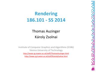
Rendering186.101 - SS2014 Thomas Auzinger Károly Zsolnai Institute of Computer Graphics and Algorithms (E186)Vienna University of Technology http://www.cg.tuwien.ac.at/staff/ThomasAuzinger.html http://www.cg.tuwien.ac.at/staff/KarolyZsolnai.html
Smallpaint features - implementation in ~250 effective lines of code, - multi-threaded rendering thanks to the OpenMP library, - some c++0x wizardry, - quasi-montecarlo sampling using low-discrepancy Halton series, - cosine importance sampling, - soft shadows, antialiasing by integrating over the screen pixels (path tracing approach), - refractions, color bleeding, caustics, - can be compiled into a binary with lesser than 4096 bytes, ...and most importantly: a great painterly look. Source: http://cg.iit.bme.hu/~zsolnai/gfx/smallpaint/index.html
Smallpaint So how is it done?
Smallpaint So how is it done? We will put into use and code what we have learned so far!
Smallpaint Code Walkthrough Vector class
Smallpaint Code Walkthrough Vector class Nothing tricky here – just the implementation of the most common operators for vectors: addition, subtraction, length (norm), dot product, cross product.
Smallpaint Code Walkthrough Representation of a ray
Smallpaint Code Walkthrough Representation of a ray The ray is given by its origin and direction. In the constructor, we initialize the direction vector to be normed, so no unpleasant surprises will happen in the calculations.
Smallpaint Code Walkthrough Objects
Smallpaint Code Walkthrough Objects An object has a color, emission, and a material type (diffuse, specular or refractive). Every kind of object has an intersection routine, and a surface normal calculation.
Smallpaint Code Walkthrough Sphere
Smallpaint Code Walkthrough Sphere
Smallpaint Code Walkthrough Sphere Why is A missing?
Smallpaint Code Walkthrough Sphere That’s why!(remember, vectors are of unit length here)
Smallpaint Code Walkthrough Sphere Discriminant
Smallpaint Code Walkthrough Sphere Discriminant vs
Smallpaint Code Walkthrough Sphere Discriminant vs Why?
Smallpaint Code Walkthrough Sphere Discriminant vs Why? Because we test if the discriminant is negative or not – we will then know if we have any real solutions. A square root won’t make any positive number negative, and 0 is invariant under the square root operator, therefore as an optimization, we postpone it after the test. The square root is expensive!
Smallpaint Code Walkthrough Sphere Discriminant vs Why? Reading: fast inverse square root hack in Quake 3: http://en.wikipedia.org/wiki/Fast_inverse_square_root
Smallpaint Code Walkthrough Sphere Plus & minus term Division by is postponed after the solution test.
Smallpaint Code Walkthrough Sphere Plus & minus term Division by is postponed after the solution test. Why?
Smallpaint Code Walkthrough Sphere Plus & minus term Division by is postponed after the solution test. Why? This is another optimization step. If the solution test returns 0 (no hit), then we don’t even need to use this division.
Smallpaint Code Walkthrough Sphere Plus & minus term Division by is postponed after the solution test. Why? Remember: if you run a profiler on a ray tracer, you’ll see that at least 90% of the execution time is spent in the intersection routines. You better push the optimization to the limit when it comes to intersecting polygons!
Smallpaint Code Walkthrough Sphere Plus & minus term Normal computation It is always pointing from the center towards the point in which we compute the normal.
Smallpaint Code Walkthrough Sphere Plus & minus term Normal computation It is always pointing from the center towards the point in which we compute the normal.
Smallpaint Code Walkthrough Sphere Plus & minus term Normal computation It is always pointing from the center towards the point in which we compute the normal.
Smallpaint Code Walkthrough Sphere Plus & minus term Normal computation It is always pointing from the center towards the point in which we compute the normal. Almost – this vector is not unit length yet. From the center to the sphere, it is a vector that has length r. We can normalize it with dividing by r instead of using the regular routine for normalizing, which includes an expensive sqrt().
Smallpaint Code Walkthrough Sphere Plus & minus term Normal computation It is always pointing from the center towards the point in which we compute the normal.
Smallpaint Code Walkthrough Sphere Plus & minus term Normal computation It is always pointing from the center towards the point in which we compute the normal. Now we got it right!
Smallpaint Code Walkthrough Perspective Camera
Smallpaint Code Walkthrough Perspective Camera
Smallpaint Code Walkthrough Perspective Camera Do you remember?(it was covered in the introduction lecture) http://cg.tuwien.ac.at/courses/Rendering/
Smallpaint Code Walkthrough Uniform sampling of a hemisphere
Smallpaint Code Walkthrough Uniform sampling of a hemisphere Reading: http://www.rorydriscoll.com/2009/01/07/better-sampling/
Smallpaint Code Walkthrough Uniform sampling of a hemisphere Reading: http://www.rorydriscoll.com/2009/01/07/better-sampling/ Intuition: Draw uniform samples on a plane and project them to the hemisphere.
Smallpaint Code Walkthrough The trace function
Smallpaint Code Walkthrough The trace function Clamping after reaching the maximum depth. Russian roulette would be the real solution!
Smallpaint Code Walkthrough The trace function Christian Machacek added Russian Roulette path termination. Thank you!
Smallpaint Code Walkthrough The trace function Terminate. Christian Machacek added Russian Roulette path termination. Thank you!
Smallpaint Code Walkthrough The trace function Continue. Christian Machacek added Russian Roulette path termination. Thank you!
Smallpaint Code Walkthrough The trace function Continue...but! Christian Machacek added Russian Roulette path termination. Thank you!
Smallpaint Code Walkthrough The trace function Continue...but!
Smallpaint Code Walkthrough The trace function Continue...but! Scale the measured radiance by the computed weight.
Smallpaint Code Walkthrough The trace function Scene intersection routine that naively intersects with every object, therefore it is linear in the number of polygons in the scene. We solve the parametric equations for t (distance), and choose the closest positive, notself-intersectingsolution. If nothing was hit, just return.
Smallpaint Code Walkthrough The trace function We make the ray of light travel towards the direction vector until the first intersection point is reached. The „hp” variable denotes the hit point. We compute the normal in this point, then set the starting point of the new ray here. We also add the emission of this object, . Disregard the „magic constant”.
Smallpaint Code Walkthrough The trace function Diffuse BRDF. We compute the next low discrepancy Halton sample, then construct a random sample, an outgoing direction on the hemisphere with uniform hemisphere sampling. This random sample is added to the normal in the intersection point. The dot product is used for light attenuation, we then trace the outgoing ray and add its contribution.
Smallpaint Code Walkthrough The trace function Specular BRDF. We have discussed handling the outgoing direction explicitly as it is described by a delta distribution. It will be set automatically to the perfect reflection direction. We also have to compute attenuation of light, and add the contribution of the outgoing ray.
Smallpaint Code Walkthrough The trace function Refractive BSDF. We invert the index of refraction upon medium change (the role of the „from” and „to” media changes), and compute the refraction direction with the vector form of Snell’s law.
Smallpaint Code Walkthrough The trace function Refractive BSDF. We invert the index of refraction upon medium change (the role of the „from” and „to” media changes), and compute the refraction direction with the vector form of Snell’s law.