Download
1 / 25
250 likes | 411 Views
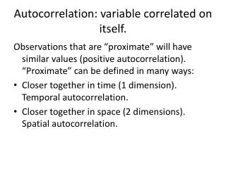
Autocorrelation: variable correlated on itself. Observations that are “proximate” will have similar values (positive autocorrelation). “Proximate” can be defined in many ways: Closer together in time (1 dimension). Temporal autocorrelation.

E N D
Autocorrelation: variable correlated on itself. Observations that are “proximate” will have similar values (positive autocorrelation). “Proximate” can be defined in many ways: • Closer together in time (1 dimension). Temporal autocorrelation. • Closer together in space (2 dimensions). Spatial autocorrelation.
Degree of autocorrelation can be calculated: • For dependent or independent variables. • For regression residuals.
Autocorrelation of regression residuals creates problem. • Usual view: estimated coefficients are unbiased, but standard errors are biased. • Alternative view: autocorrelated residuals signal presence of omitted variables. estimated coefficients are biased.
Residuals: Hedonic House Price Model (Blue paid too little; Red paid too much)
International Data • Can see spatial autocorrelation in international data: neighboring countries tend to have similar values. • Not only physical proximity, but also cultural proximity, will lead to similar values.
Cultural proximity can be defined using a language phylogeny.
The 12 selected languages are on the periphery of the digraph. Links point toward higher taxonomic levels, with all nodes ultimately connected to the node labeled Indo-European. The numbers indicate for selected nodes the maximum path length leading to that node. The taxonomy is from Grimes 2000
Standard Cross-Cultural Sample • World divided up into “culture regions,” one well-documented society picked from each of these, for total of 186 societies. • Over 2,000 variables gradually added. • Full range of human societies, so that any statement that claims to hold universally for humans can be tested.
Larger and darker circles for societies in which gods support human morality; smallest and lightest are societies in which gods are uninvolved in human affairs. Cyan triangles are missing values.
% married women in monogamous marriages, by major language phylum and by religion
Galton’s problem Observations not independent. • Common descent (language phylogeny) • Cultural borrowing (geographic distance, religion phylogeny) In regression context, Galton’s problem will cause biased coefficients and biased standard errors.
Galton’s problem example: Hypothesis: Drinking alcohol dampens the libido of religious specialists. alcohol wives Ecuador 1 0 Iran 0 2 Ireland 1 0 Morocco 0 3 Spain 1 0 Yemen 0 4 Pearson correlation= -0.9332565, p-value=0.0065 Adapted from Victor de Munck and Andrey Korotayev. 2000. “Cultural Units in Cross-Cultural Research.“ Ethnology 39(4): 335-348 An observed correlation between a pair of cultural traits across cultures could be due to the borrowing of the traits, as a package, from a common source (“horizontal transmission”), or could be due to their transmission, as a package, from a common ancestor (“vertical transmission”), or could be due to a true functional relationship.
Correcting for Galton’s problem (continued) Problem: The spatial weight matrices WR, WL and WD will be correlated with each other (societies with similar languages are usually physically proximate and have similar religions, as well), so that there is an identification problem with more than one spatial lag term. Solution: Create a new spatial matrix Woptimal= d*WD + r*WR + l*WL , where d+r+l=1. Make all possible matrices Woptimal using values (0,0.05,0.10,0.15,… , 0.85,0.90,0.95,1) for each of the weights (d,r,l). Estimate the model using each of the (211) weight matrices, recording the model R2. Retain the spatial weight matrix Woptimal which explains the highest variation of the dependent variable.