Download
1 / 25
250 likes | 377 Views
UV ENVIRONMENT OF EXOPLANETS. Jeffrey Linsky, Kevin France, and Rachel Bushinsky University of Colorado Boulder Colorado ExoClimes 2012 Aspen Colorado 15-20 Jan 2012.

E N D
UV ENVIRONMENT OF EXOPLANETS Jeffrey Linsky, Kevin France, and Rachel Bushinsky University of Colorado Boulder Colorado ExoClimes 2012 Aspen Colorado 15-20 Jan 2012
Simulated spectrum of GJ 436 (M2.5 V with a 0.073MJ exoplanet). Note emission lines and photo-absorption cross-sections of H2O and CH4
COS spectrum of 2M1207 a young M8 brown dwarf with a CS disk (H2) and accretion (C IV) but no Si III-IV or Mg II emission lines (France et al. ApJ 715, 596 (2010))
HST/STIS spectrum of AU Mic (M1 V) (Pagano et al. ApJ 532, 497 (2000). What line emits most of the UV flux?
UV spectra of solar-mass stars (spectral types G0-G2 dwarfs)
“Sun in time Project”. Fluxes at 1 AU from solar type stars as a function of age (Ribas et al. ApJ 622, 680 (2005)). Flux is very sensitive to age (activity) at shorter wavelengths.
Spectral flux (for solar type stars) decreases with age most rapidly at the shortest wavelengths. Is the same true for M dwarfs?
Reconstructing Lyman-α Line Profiles Using Information on the Local ISM (Wood et al. ApJS 159, 118 (2005). Left: ξ Boo A (G8 V). Right: AD Leo (M3.5 V) and AU Mic (M0 V).
Observed and reconstructed Lyman-α line profiles (Wood et al. ApJS 159, 118 (2005)
Limitations on the Lyman-α line reconstruction technique • Must be able to resolve the D I Lyman-α line to reconstruct the H I line. • Effective horizon at log N(HI)=18.7 (15-100 pc). • Should also have high resolution spectra of metal lines (e.g., MgII or FeII) to determine whether many velocity components in the line of sight. Curves for increasing HI column density are for log N(HI) = 17.5, 17.8, 18.1, 18.4, 18.7. Solid and dashed lines are for T=10,000 and 5,000 K. (Wood et al. 2005)
Observed and reconstructed Lyman-α flux for GJ667C (M1.5V) 2 exoplanets at 0.05 and 0.12 AU.
HST observations of M dwarfs with exoplanets (programs 12034, 12035, and 12464)
Maps of n(HI) computed in hydrodynamic models of stellar atmospheres (Wood et al 2005). Scales are in AU. Solid line indicates LOS to the observer. 61 Vir has 3 exoplanets located inside of its hydrogen wall.
Interstellar, astrospheric, and heliospheric Lyman-α absorption • Interstellar gas flow from above. • Line of sight passes through astrosphere, ISM, and then heliosphere • Astrospheric absorption is blue compared to ISM because H slows down in the astropause as seen by the star. • Heliospheric absorption is red compared to ISM because H slows down in the heliopause. • Astrospheric absorption proportional to stellar mass loss rate.
Measuring stellar mass loss rates from the astrospheric absorption feature on the blue side of interstellar Lyman-α absorption
Mass loss rate vs activity (X-ray surface flux) and stellar age • Solid dots indicate dwarf stars (Prox Cen and EV Lac are only M dwarfs). • Near Fx=106 there is a break suggesting a change in magnetic field structure. • More measurements are needed (HST GO-19 proposal). • Ṁ ~ FX1.34±0.18 ~ t2.33±0.55
Conclusions • Stellar UV+FUV+EUV flux incident on an exoplanet’s atmosphere photodissociates important molecules like H2O and CH4 and photoionizes important atoms like H and O. • Reconstructed Lyman-α dominates the UV flux often by a very large factor. • Lyman-α and UV stellar fluxes for G stars follow a regular dependence on B-V and rotation period (a proxy for stellar activity). • Lyman-α and UV fluxes of M stars cannot be easily predicted and must be observed. We have HST observing programs for M stars with exoplanets. • We have found a scaling law for stellar mass loss rates which important for computing charge exchange rates. We have an HST/STIS observing program to extend this to M dwarfs.
We are now writing HST proposals for new observations of M dwarfs with exoplanets Those interested in providing data for new targets or in theoretical analysis (e.g., atmospheric chemistry calculations) are welcome to join the proposing team. Please see me.