Multiple Choice Practice
E N D
Presentation Transcript
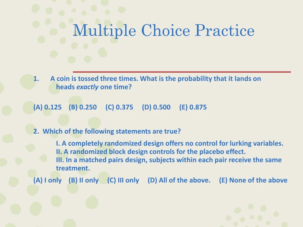
Multiple Choice Practice • A coin is tossed three times. What is the probability that it lands on headsexactly one time? (A) 0.125 (B) 0.250 (C) 0.375 (D) 0.500 (E) 0.875 2. Which of the following statements are true? I. A completely randomized design offers no control for lurking variables. II. A randomized block design controls for the placebo effect. III. In a matched pairs design, subjects within each pair receive the same treatment. (A) I only (B) II only (C) III only (D) All of the above. (E) None of the above
Solutions • The correct answer is (C). Sample Space: HHH, HHT, HTH, THH, HTT, THT, TTH, and TTT. Of the eight possible outcomes, three have exactly one head. • The correct answer is (E). In a completely randomized design , subjects are randomly assigned to treatment conditions. Randomization provides some control for lurking variables . By itself, a randomized block design does not control for the placebo effect . To control for the placebo effect, the experimenter must include a placebo in one of the treatment levels. In a matched pairs design , subjects within each pair are assigned to different treatment levels.
Chap 6.1 Discrete and Continuous Random Variables
Random Variable • Takes a numerical value that describes an outcome of a random phenomenon • Usually represented by capital letters near the end of the alphabet (X, Y, Z)
Probability Distribution of a Random Variable (X) • Gives the possible values and their probabilities
Discrete Random Variable • Has a finitely many possible values. • All outcomes can be listed • Each probability must be between 0 and 1 • Sum of the probabilities is 1
Mean of a Discrete Random Variable(Expected Value) • Analyzing discrete random variables: SOCS • Mean of any discrete random variable is an average of the possible outcomes, with each outcome weighted by its probability.
Mean of a Discrete Random Variable(Expected Value) • To find the mean (or expected value) of “”, multiply each possible value by its probability, then add all the products
ExampleGetting good grades • Stats 101, fall 2003, grade distribution: • 21% A’s, 43% B’s, 30% C’s, 5% D’s, 1% F’s • A student is chosen at random from this class (each student has the same probability of being chosen) • Let X = student’s grade (A=4, B=3, C=2, D=1, F=0)
Probability distribution of Grades: Probability of getting a B or better? 0.64 Compute the mean of the random variable.
Variance and Standard Dev. of Discrete Random Variable • Variance • Standard Deviation • Compute and interpret the standard deviation for our Stat 101 Grades example.
Continuous Random Variable • Takes all values in an interval of numbers • Described by a density curve • Cannot list all outcomes • Probability distributions are described by a density curve • Assign probability 0 to every individual outcome. • No distinction between ≥ and >
Normal Distribution • Are one type of continuous probability distribution. • Normal curve is most popular density curve • N(µ, σ): is a normal random variable having distribution N(0,1)
Example: Normal probability distributions The heights of young women closely follow the Normal distribution with mean µ = 64 inches and standard deviation σ = 2.7 inches. Now choose one young woman at random. Call her height Y. If we repeat the random choice very many times, the distribution of values of Y is the same Normal distribution that describes the heights of all young women. Problem: What’s the probability that the chosen woman is between 68 and 70 inches tall?
Example: Normal probability distributions State the distribution and the values of interest. The height Y of a randomly chosen young woman has the N(64, 2.7) distribution. We want to find P(68 ≤ Y ≤ 70). Perform calculations—show your work! The standardized scores for the two boundary values are
Assignment6.1 Pg. 359 #3-7 odd, 11, 14-15, 21-25 odd, 27-30all
