EE 122 : Shortest Path Routing
480 likes | 684 Views
EE 122 : Shortest Path Routing. Ion Stoica TAs: Junda Liu, DK Moon, David Zats http://inst.eecs.berkeley.edu/~ee122/fa09 (Materials with thanks to Vern Paxson , Jennifer Rexford, and colleagues at UC Berkeley). What is Routing?. Routing implements the core function of a network:

EE 122 : Shortest Path Routing
E N D
Presentation Transcript
EE 122: Shortest Path Routing Ion Stoica TAs: Junda Liu, DK Moon, David Zats http://inst.eecs.berkeley.edu/~ee122/fa09 (Materials with thanks to Vern Paxson, Jennifer Rexford,and colleagues at UC Berkeley)
What is Routing? Routing implements the core function of a network: It ensures that information accepted for transfer at a source node is delivered to the correct set of destination nodes, at reasonable levels of performance.
Internet Routing • Internet organized as a two level hierarchy • First level – autonomous systems (AS’s) • AS – region of network under a single administrative domain • AS’s run an intra-domain routing protocols • Distance Vector, e.g., Routing Information Protocol (RIP) • Link State, e.g., Open Shortest Path First (OSPF) • Between AS’s runs inter-domain routing protocols, e.g., Border Gateway Routing (BGP) • De facto standard today, BGP-4
Example Interior router BGP router AS-1 AS-3 AS-2
Forwarding vs. Routing • Forwarding: “data plane” • Directing a data packet to an outgoing link • Individual router using a forwarding table • Routing: “control plane” • Computing paths the packets will follow • Routers talking amongst themselves • Individual router creating a forwarding table
Link State Routing E.g. Algorithm: Dijkstra E.g. Protocol: OSPF Distance Vector Routing E.g. Algorithm: Bellman-Ford E.g. Protocol: RIP Know Thy Network • Routing requires knowledge of the network structure • Centralized global state • Single entity knows the complete network structure • Can calculate all routes centrally • Problems with this approach? • Distributed global state • Every router knows the complete network structure • Independently calculates routes • Problems with this approach? • Distributed no-global state • Every router knows only about its neighboring routers • Independently calculates routes • Problems with this approach?
5 3 5 2 2 1 3 1 2 1 C D A B E F Modeling a Network • Modeled as a graph • Routers nodes • Link edges • Possible edge costs • delay • congestion level • Goal of Routing • Determine a “good” path through the network from source to destination • Good usually means the shortest path
Host C Host D Host A N2 N1 N3 N5 Host B Host E N4 N6 N7 Link State: Control Traffic • Each node floods its local information to every other node in the network • Each node ends up knowing the entire network topology use Dijkstra to compute the shortest path to every other node
C C C C C C C A A A A A A A D D D D D D D Host C Host D Host A B B B B B B B E E E E E E E N2 N1 N3 N5 Host B Host E N4 N6 N7 Link State: Node State
c(i,j): link cost from node i to j; cost infinite if not direct neighbors; ≥ 0 D(v): current value of cost of path from source to destination v p(v): predecessor node along path from source to v, that is next to v S: set of nodes whose least cost path definitively known D C A E B F 5 3 5 2 2 1 3 1 2 1 Notation Source
Dijsktra’s Algorithm • c(i,j): link cost from node i to j • D(v): current cost source v • p(v): predecessor node along path from source to v, that is next to v • S: set of nodes whose least cost path definitively known 1 Initialization: 2 S = {A}; 3 for all nodes v 4 if v adjacent to A 5 then D(v) = c(A,v); 6 else D(v) = ; 7 8 Loop 9 find w not in S such that D(w) is a minimum; 10 add w to S; 11 update D(v) for all v adjacent to w and not in S: 12 if D(w) + c(w,v) < D(v) then // w gives us a shorter path to v than we’ve found so far 13 D(v) = D(w) + c(w,v); p(v) = w; 14 until all nodes in S;
D C A E B F 5 3 5 2 2 1 3 1 2 1 Example: Dijkstra’s Algorithm D(B),p(B) 2,A D(D),p(D) 1,A D(C),p(C) 5,A D(E),p(E) Step 0 1 2 3 4 5 start S A D(F),p(F) 1 Initialization: 2 S = {A}; 3 for all nodes v 4 if v adjacent to A 5 then D(v) = c(A,v); 6 else D(v) = ; …
… • 8 Loop • 9 find w not in Ss.t. D(w) is a minimum; • 10 add w to S; • update D(v) for all v adjacent • to w and not in S: • If D(w) + c(w,v) < D(v) then • D(v) = D(w) + c(w,v); p(v) = w; • 14 until all nodes in S; D C A E B F 5 3 5 2 2 1 3 1 2 1 Example: Dijkstra’s Algorithm D(B),p(B) 2,A D(D),p(D) 1,A D(C),p(C) 5,A D(E),p(E) Step 0 1 2 3 4 5 start S A D(F),p(F)
… • 8 Loop • 9 find w not in S s.t. D(w) is a minimum; • 10 add w to S; • update D(v) for all v adjacent • to w and not in S: • If D(w) + c(w,v) < D(v) then • D(v) = D(w) + c(w,v); p(v) = w; • 14 until all nodes in S; C D E A B F Example: Dijkstra’s Algorithm D(B),p(B) 2,A D(D),p(D) 1,A D(C),p(C) 5,A D(E),p(E) Step 0 1 2 3 4 5 start S A AD D(F),p(F) 5 3 5 2 2 1 3 1 2 1
… • 8 Loop • 9 find w not in S s.t. D(w) is a minimum; • 10 add w to S; • update D(v) for all v adjacent • to w and not in S: • If D(w) + c(w,v) < D(v) then • D(v) = D(w) + c(w,v); p(v) = w; • 14 until all nodes in S; C D E A B F Example: Dijkstra’s Algorithm D(B),p(B) 2,A D(D),p(D) 1,A D(C),p(C) 5,A 4,D D(E),p(E) 2,D Step 0 1 2 3 4 5 start S A AD D(F),p(F) 5 3 5 2 2 1 3 1 2 1
… • 8 Loop • 9 find w not in S s.t. D(w) is a minimum; • 10 add w to S; • update D(v) for all v adjacent • to w and not in S: • If D(w) + c(w,v) < D(v) then • D(v) = D(w) + c(w,v); p(v) = w; • 14 until all nodes in S; C D E A B F Example: Dijkstra’s Algorithm D(B),p(B) 2,A D(D),p(D) 1,A D(C),p(C) 5,A 4,D 3,E D(E),p(E) 2,D Step 0 1 2 3 4 5 start S A AD ADE D(F),p(F) 4,E 5 3 5 2 2 1 3 1 2 1
… • 8 Loop • 9 find w not in S s.t. D(w) is a minimum; • 10 add w to S; • update D(v) for all v adjacent • to w and not in S: • If D(w) + c(w,v) < D(v) then • D(v) = D(w) + c(w,v); p(v) = w; • 14 until all nodes in S; C D E A B F Example: Dijkstra’s Algorithm D(B),p(B) 2,A D(D),p(D) 1,A D(C),p(C) 5,A 4,D 3,E D(E),p(E) 2,D Step 0 1 2 3 4 5 start S A AD ADE ADEB D(F),p(F) 4,E 5 3 5 2 2 1 3 1 2 1
… • 8 Loop • 9 find w not in S s.t. D(w) is a minimum; • 10 add w to S; • update D(v) for all v adjacent • to w and not in S: • If D(w) + c(w,v) < D(v) then • D(v) = D(w) + c(w,v); p(v) = w; • 14 until all nodes in S; C D E A B F Example: Dijkstra’s Algorithm D(B),p(B) 2,A D(D),p(D) 1,A D(C),p(C) 5,A 4,D 3,E D(E),p(E) 2,D Step 0 1 2 3 4 5 start S A AD ADE ADEB ADEBC D(F),p(F) 4,E 5 3 5 2 2 1 3 1 2 1
… • 8 Loop • 9 find w not in S s.t. D(w) is a minimum; • 10 add w to S; • update D(v) for all v adjacent • to w and not in S: • If D(w) + c(w,v) < D(v) then • D(v) = D(w) + c(w,v); p(v) = w; • 14 until all nodes in S; C D E A B F 5 3 5 2 2 1 3 1 2 1 Example: Dijkstra’s Algorithm D(B),p(B) 2,A D(D),p(D) 1,A D(C),p(C) 5,A 4,D 3,E D(E),p(E) 2,D Step 0 1 2 3 4 5 start S A AD ADE ADEB ADEBC ADEBCF D(F),p(F) 4,E
D C A E B F 5 3 5 2 2 1 3 1 2 1 Example: Dijkstra’s Algorithm D(B),p(B) 2,A D(D),p(D) 1,A D(C),p(C) 5,A 4,D 3,E D(E),p(E) 2,D Step 0 1 2 3 4 5 start S A AD ADE ADEB ADEBC ADEBCF D(F),p(F) 4,E To determine path A C (say), work backward from C via p(v)
D C A E B F 5 3 5 2 2 1 3 1 2 1 The Forwarding Table • Running Dijkstra at node A gives the shortest path from A to all destinations • We then construct the forwarding table
Complexity • How much processing does running the Dijkstra algorithm take? • Assume a network consisting of N nodes • Each iteration: need to check all nodes, w, not in S • N(N+1)/2 comparisons: O(N2) • More efficient implementations possible: O(N log(N))
X A X A C B D C B D (a) (b) X A X A C B D C B D (c) (d) Obtaining Global State • Flooding • Each router sends link-state information out its links • The next node sends it out through all of its links • except the one where the information arrived • Note: need to remember previous msgs & suppress duplicates!
Flooding the Link State • Reliable flooding • Ensure all nodes receive link-state information • Ensure all nodes use the latest version • Challenges • Packet loss • Out-of-order arrival • Solutions • Acknowledgments and retransmissions • Sequence numbers • Time-to-live for each packet
When to Initiate Flooding • Topology change • Link or node failure • Link or node recovery • Configuration change • Link cost change • See next slide for hazards of dynamic link costs based on current load • Periodically • Refresh the link-state information • Typically (say) 30 minutes • Corrects for possible corruption of the data
e C C C C D D D D A A B A B B B A 0 2+e 2+e 2+e 0 0 0 0 1 1 1+e 1+e 1 1+e 0 e 0 0 … recompute … recompute routing … recompute Oscillations • Assume link cost = amount of carried traffic 1 1+e 0 0 e 0 1 1 initially • How can you avoid oscillations?
5 Minute Break Questions Before We Proceed?
Distance Vector Routing • Each router knows the links to its immediate neighbors • Does not flood this information to the whole network • Each router has some idea about the shortest path to each destination • E.g.: Router A: “I can get to router B with cost 11 via next hop router D” • Routers exchange this information with their neighboring routers • Again, no flooding the whole network • Routers update their idea of the best path using info from neighbors
Host C Host D Host A N2 N1 N3 N5 Host B Host E N4 N6 N7 Information Flow in Distance Vector
Bellman-Ford Algorithm • INPUT: • Link costs to each neighbor • Not full topology • OUTPUT: • Next hop to each destination and the corresponding cost • Does not give the complete path to the destination
C D B A Bellman-Ford - Overview • Each router maintains a table • Row for each possible destination • Column for each directly-attached neighbor to node • Entry in row Y and column Z of node X best known distance from X to Y, via Z as next hop = DZ(X,Y) Neighbor (next-hop) Node A 3 2 1 1 7 Destinations DC(A, D)
C D B A Bellman-Ford - Overview • Each router maintains a table • Row for each possible destination • Column for each directly-attached neighbor to node • Entry in row Y and column Z of node X best known distance from X to Y, via Z as next hop = DZ(X,Y) Node A 3 2 1 1 7 Smallest distance in row Y = shortest Distance of A to Y, D(A, Y)
wait for (change in local link cost or msg from neighbor) recompute distance table if least cost path to any dest has changed, notify neighbors Each node: Bellman-Ford - Overview • Each router maintains a table • Row for each possible destination • Column for each directly-attached neighbor to node • Entry in row Y and column Z of node X best known distance from X to Y, via Z as next hop = DZ(X,Y) • Each local iteration caused by: • Local link cost change • Message from neighbor • Notify neighbors only if least cost path to any destination changes • Neighbors then notify their neighbors if necessary
Distance Vector Algorithm (cont’d) 1 Initialization: 2 for all neighbors V do 3 ifV adjacent to A 4 D(A, V) = c(A,V); else D(A, V) = ∞; send D(A, Y) to all neighbors loop: 8 wait (until A sees a link cost change to neighbor V /* case 1 */ 9 or until A receives update from neighbor V) /* case 2 */ 10 if (c(A,V) changes by ±d) /* case 1 */ 11 for all destinations Y that go through Vdo 12 DV(A,Y) = DV(A,Y) ± d 13 else if (update D(V, Y) received from V) /* case 2 */ /* shortest path from V to some Y has changed */ 14 DV(A,Y) = DV(A,V) + D(V, Y); /* may also change D(A,Y) */ 15 if (there is a new minimum for destination Y) 16 send D(A, Y) to all neighbors 17 forever • c(i,j): link cost from node i to j • DZ(A,V): cost from A to V via Z • D(A,V): cost of A’s best path to V
C D B A Example:1st Iteration (C A) Node A Node B 3 2 1 1 7 DC(A, B) = DC(A,C) + D(C, B) = 7 + 1 = 8 DC(A, D) = DC(A,C) + D(C, D) = 7 + 1 = 8 Node C Node D • loop: • … • 13 else if (update D(A, Y) fromC) • 14 DC(A,Y) = DC(A,C) + D(C, Y); • 15 if (new min. for destination Y) • 16 send D(A, Y) to all neighbors • 17 forever
C D B A Example: 1st Iteration (B A) Node A Node B 3 2 1 1 7 DB(A, C) = DB(A,B) + D(B, C) = 2 + 1 = 3 DB(A, D) = DB(A,B) + D(B, D) = 2 + 3 = 5 Node C Node D • loop: • … • 13 else if (update D(A, Y) fromB) • 14 DB(A,Y) = DB(A,B) + D(B, Y); • 15 if (new min. for destination Y) • 16 send D(A, Y) to all neighbors • 17 forever
C D B A Example:End of 1st Iteration Node A Node B 3 2 1 1 7 Node C Node D End of 1st Iteration All nodes knows the best two-hop paths
C D B A Example:2nd Iteration (A B) Node A Node B 3 2 1 1 7 DA(B, C) = DA(B,A) + D(A, C) = 2 + 3 = 5 DA(B, D) = DA(B,A) + D(A, D) = 2 + 5 = 7 Node C Node D • loop: • … • 13 else if (update D(B, Y) fromA) • 14 DA(B,Y) = DA(B,A) + D(A, Y); • 15 if (new min. for destination Y) • 16 send D(B, Y) to all neighbors • 17 forever
C D B A Example:End of 2nd Iteration Node A Node B 3 2 1 1 7 Node C Node D End of 2nd Iteration All nodes knows the best three-hop paths
C D B A Example:End of 3rd Iteration Node A Node B 3 2 1 1 7 Node C Node D End of 2nd Iteration: Algorithm Converges!
C A B Link cost changes here Algorithm terminates Distance Vector: Link Cost Changes loop: 8 wait (until A sees a link cost change to neighbor V 9 or until A receives update from neighbor V) / 10 if (c(A,V) changes by ±d) /* case 1 */ 11 for all destinations Y that go through Vdo 12 DV(A,Y) = DV(A,Y) ± d 13 else if (update D(V, Y) received from V) /* case 2 */ 14 DV(A,Y) = DV(A,V) + D(V, Y); 15 if (there is a new minimum for destination Y) 16 send D(A, Y) to all neighbors 17 forever 1 4 1 50 Node B “good news travels fast” Node C time
C A B Distance Vector: Count to Infinity Problem loop: 8 wait (until A sees a link cost change to neighbor V 9 or until A receives update from neighbor V) / 10 if (c(A,V) changes by ±d) /* case 1 */ 11 for all destinations Y that go through Vdo 12 DV(A,Y) = DV(A,Y) ± d 13 else if (update D(V, Y) received from V) /* case 2 */ 14 DV(A,Y) = DV(A,V) + D(V, Y); 15 if (there is a new minimum for destination Y) 16 send D(A, Y) to all neighbors 17 forever 60 4 1 50 “bad news travels slowly” Node B Node C … time Link cost changes here
60 4 1 50 C A B Distance Vector: Poisoned Reverse • If B routes through C to get to A: • Btells C its (B’s) distance to A is infinite (so C won’t route to A via B) • Will this completely solve count to infinity problem? Node B Node C time Link cost changes here; C updates D(C, A) = 60 as Bhas advertised D(B, A) = ∞ Algorithm terminates
Routing Information Protocol (RIP) • Simple distance-vector protocol • Nodes send distance vectors every 30 seconds • … or, when an update causes a change in routing • Link costs in RIP • All links have cost 1 • Valid distances of 1 through 15 • … with 16 representing infinity • Small “infinity” smaller “counting to infinity” problem • RIP is limited to fairly small networks • E.g., campus
Per-nodemessagecomplexity: LS: O(e) messages e: number of edges DV: O(d) messages, many times d is node’s degree Complexity/Convergence LS: O(N log N) computation Requires global flooding DV: convergence time varies Count-to-infinity problem Robustness: what happens if router malfunctions? LS: Node can advertise incorrect link cost Each node computes only its own table DV: Node can advertise incorrect path cost Each node’s table used by others; errors propagate through network Link State vs. Distance Vector
Summary • Routing is a distributed algorithm • Different from forwarding • React to changes in the topology • Compute the shortest paths • Two main shortest-path algorithms • Dijkstra link-state routing (e.g., OSPF, IS-IS) • Bellman-Ford distance-vector routing (e.g., RIP) • Convergence process • Changing from one topology to another • Transient periods of inconsistency across routers • Next time: BGP • Reading: K&R 4.6.3