Download
1 / 25

E N D
Inventory Firms ultimately want to sell consumers output in the hopes of generating a profit. Along the way to having the output available inventory can occur in several ways. There can be an inventory of raw material as it is waiting to be processed, there can be an inventory of partially completed output and there can be completed output not yet sold to the customer. In other words, there can be inventory throughout the supply chain.
Reasons to carry inventory 1) To protect against uncertainties, 2) To allow economic production and purchase, 3) To cover anticipated changes in demand or supply, and 4) To provide for transit. So, carrying inventories of inputs or output can make production flows more even and can allow for more economical lot processing and purchase discounts.
Cost Structures Here we want to consider the various types of costs associated with inventory. 1) Item costs are the costs of buying or producing the item. This cost is usually expressed as a per unit cost (on average) and multiplied by the number of units involved. 2) Ordering or setup costs do Not depend on the number of items ordered. These costs are assigned to the entire batch and include costs of typing order and transportation costs. 3) Carrying or holding costs are made up of cost of capital, cost of storage and costs of obsolescence, deterioration and loss and these costs are typically counted as a percentage of the dollar volume of inventory. For example, a 15% holding cost means you take .15 times the dollar amount in inventory as the cost.
Cost Structures 4) Stockout costs are essentially the cost of losing current and or future business because items were not on hand when desired. Some of the costs mentioned here exhibit trade-offs. What I mean by this is that if we raise one type of cost we lower another type. As an example, as we increase the size of inventory and thus storage cost the stockout cost is lowered. With these ideas in mind we next study the economic order quantity model (EOQ). Note the assumptions of the model listed on page 348. In particular note demand has a constant rate and items are ordered in a fixed lot size.
EOQ In this model the total cost is made up of ordering cost plus carrying cost per year. The idea is to pick an order size, Q, that leads to the lowest total cost. Ordering costs per year = cost per order times orders per year. If D = the total demand in a year and Q is the amount ordered each time, then D/Q = the number of orders per year. With S the cost of placing an order, the ordering cost per year is S(D/Q). Carrying cost per year = annual carrying rate times unit cost times average inventory. Q/2 is the average inventory because at the beginning of the order period you have Q and at the end you have 0, (Q + 0)/2 = Q/2. We assume no quantity discounts so the unit cost will be called C and i is the carrying rate. Thus, the carrying cost = i(C)(Q/2).
EOQ Total cost = ordering cost + carrying cost = S(D/Q) + i(C)(Q/2) Now, we have said demand D is constant through the year. Thus the more that is ordered, Q, the less orders can be placed in the year. Thus, the higher the Q the lower the ordering cost. But, if Q is higher the carrying costs are higher. Thus we see a trade-off. When Q goes up order costs fall but carrying costs rise. Some really smart folks (Wilson and Harris) found the Q to order to give the lowest cost is Q = square root(2SD/iC).
EOQ Example Say a carpet store has demand for a certain type of carpet = 360 yards per year = D, it has a $10 cost per order = S, it as a 25% carrying cost = i, and the unit cost is $8 per yard = C. Thus the EOQ = Q = sqrt[{(2)(10)(360)}/{(.25)(8)}] = 60. Since the demand is 360 per year and it will order 60 units at a time it will order 360/60 = 6 times per year. Its total cost will be 10(360/60) + .25(8)(60/2) = 60 + 60 = 120. Just to show that this is the lowest TC, pick another Q (not using the EOQ formula) and see what is TC. I’ll try 40. TC = 10(360/40) + .25(8)(40/2) = 90 + 40 = 130. So, if you order less in an order you have to order more per year to meet the 360 level of demand. Order costs are higher but carrying costs shrink.
EOC example If you look at ordering 90 at a time you get TC = 10(360/90) + .25(8)(90/2) = 40 + 90. Thus, if a lot is ordered at one time you make fewer orders but you have a larger carrying cost. The EOQ formula shows us the Q that minimizes the total cost during the year.
Continuous Review or Q System The EOQ model is based on several assumptions, one being that there is a constant demand. This may not be realistic. Next we consider some models that allow demand to occur more at random. In the EOQ model once the best order size, Q, was determined, the firm would order at a regular interval that divided the period (year) up into D/Q times. So, the same amount was ordered at the same interval. In the Q system we will study the same amount will be ordered at different intervals of time. Then, in the P system (I say more later) different amounts will be ordered at a fixed time interval. The Q system relies on the normal distribution, so we turn there next.
Q System Say daily demand is normal with mean = 200 and standard deviation = 150. Then we might have a question like, “what is the probability daily demand will be 350, or less?” 200 350 daily demand To answer the question we see the normal distribution and we have to find the area under the curve to the left of 350. We resort to a z calculation = (value (like 350) minus mean)/st dev. Our z = (350 – 200)/150 = 1.00 (usually we round z to 2 decimals). Then we go to a z table and see the value with z = 1.00 of .8413 (really .5 + .3413) and we say the probability is 84.13.
Q System Page 354 has a table that rounds z to 1 decimal and the service level is 84.1 (84.13 rounded to 1 decimal). So this table really has an abbreviated version of the z table. Now, when orders are placed to replenish inventory, it takes some number of days for the order to arrive. If demand during this lead time is higher than our trigger reorder level R (the level such that when our inventory reaches this level an order of Q Will be made), the demand will not be met and we say there is a stockout. If demand is less than this trigger reorder level then demand will be met and we can calculate the fill rate or service level as the percentage of customer demand satisfied by inventory.
Q System Before we had an example of daily demand being normal with mean = 200 and standard deviation = 150. Now, if the lead time is 4 days, then the demand during the 4 days of lead time will be normal with mean = 4 times daily mean demand of 200 = 800 and standard deviation = sqrt(4 days)times daily standard deviation of 150 = 300. On the next slide I show a normal distribution with mean of 800 and a standard deviation of 300. We will use this graph and related ideas to help us determine what the trigger reorder amount R should be.
Q System 800 950 1100 1400 demand over lead time Say in general the mean demand over the lead time period is m, which equals 800 here. For a while I am just going to play a hypothetical game. I am going to ask what would happen if our trigger order amount R is various amounts. In fact I will look at the cases where R = 800, R = 950, R = 1100 and R =1400. Let’s do this next, but refer back to this slide to “see” what is going on.
Q System Say we make R = 1400, meaning that if our stock position reaches R we will reorder some amount (I will say how much to order later). Since our lead time here is 4 days this will mean that over the next 4 days if actual demand is 1400 or less than we will have enough inventory to meet the demand. But, if actual demand is over 1400 we will not have enough on hand and there will be a stockout. (Have you ever gone to a store to buy something, maybe it was even advertised, and the store ran out? How do you feel at that point? Are you bummed out, upset or just plain seething with anger? Stores do not what to bum you out, but schtuff happens!)
Q System Since demand is random, and here assumed normal, we can calculate what percentage of the time demand will be above or below the trigger amount R, here picked to be 1400. The z for 1400 is (1400 – 800)/300 = 2.0. The table on page 354 tells us in this case we would meet demand 97.7 percent of the time. Thus our service level or fill rate would be that we meet 97.7 percent of customer demand from inventory. Similarly, 100 – 97.7 = 2.3 percent of the time we would have a stockout. If R = 1100, z = (1100 – 800)/300 = 1.0 and the service level will be 84.1% and the stockout % will be 15.9%. If R = 950, z = (950 – 800)/300 = .5 and the service level will be 69.1% and the stockout % will be 30.9%. If R = 800, z =(800 – 800)/300 = 0 and the service level will be 50% and the stockout % will be 50%
Q System What I have done here is talk about hypothetical R values, levels of the stock position that would trigger an order be made. With different R values we see different service levels and stockout %’s. We could work in reverse to what I have presented. If demand over lead time has mean = 800 and standard deviation = 300, what should R be to make the service level 97.7? The z there is 2.0. Thus 2.0 = (R – 800)/300 and solving for R we get R = 800 + 2.0(300) = 1400. In general, R = m + zσ = mean over lead time + safety stock. Thus, we need to think about how serious our customers become if there is a stock out. The more serious the higher the service level should be and thus the higher the z we pick.
Q System I mentioned before I would say how much should be ordered. Just order the EOQ on a yearly average demand basis. Thus, if average demand is 200 per day, and say we are open 5 days a week for 50 weeks then annual average demand is 250(5)(50) = 50,000 units per year. If S = $20 per order, i = 20% per year and C = $10 per unit, the the EOQ Q = sqrt[{2(20)(50000)}/{.2(10)}] = sqrt(1000000) = 1000. So, 1000 units would be ordered when R is reached. Since annual demand has an average of 50,000 and we order in lots of 1000 we will make an average of 50 orders per year. Since there are 250 working days in the year orders will be made on average every 250/50 = 5 days.
Q System What should R be if you want a service level of 95.0? Note 95.0 is not in the table on page 354, but it is in the middle of 94.5 and 95.5 so we take the z in the middle of the associated z’s for a z = 1.65. R = 800 + 1.65(300) = 1295. The order amount R depends of the service level desired. The Q amount to order still is picked by the EOQ method, but using annual average demand.
Review Review: In the EOQ model we order the same amount at essentially the same interval of time. In the Q System we order the EOQ amount each time but order it when the stock position reaches a “trigger” level R. R will depend on actual demand. In the P System we order at a regular interval P(maybe because a delivery truck always stops by on a regular interval), but we order an amount so that our stock position gets up to a target level T. Recall the EOQ formula Q = Sqrt[{2(S)(D)}/{i(c)}]. Remember this is how much of the annual demand should be ordered when an order is made under EOQ or the Q System.
P System With Q ordered each time and an average daily demand amount, the review period should be P = Q from EOQ divided by average daily demand. So, an order will be placed every P days. Remember that once an order is placed it will take L days to arrive. Say P = 5 and L = 4. Say on day 1 an order is placed. Once that order is placed it is included in the stock position. The target level T has to be such that on day 1 after the order is placed enough inventory will be around to get us to the next review period and the lead time of that delivery. So our target inventory level should get us through P + L days.
P System The target inventory should then equal Average daily demand times (P + L) + z (sqrt(P + L)) standard deviation of daily demand. Example: Let’s use the same example as used in the Q system – that one started on page 354 EOQ Q = 1000 cases P is then 1000/200 = 5. L is stated as 4. Average daily demand is stated as 200. The standard deviation of daily demand is 150. Recall z is based on a service level desired and if we want 95% service level we use z = 1.65. Thus the target inventory level is 200(9) + 1.65(sqrt(9))(150 ) = 1800 + 1.65(3)(150) = 2542
P System So, in our example the target inventory level is 2542. But this is not the amount to order each time. The amount to order is this target minus the stock position at the time of the order. This amount will differ from order to order because the demand is not constant, but random. So, if the stock position is already 1756 the order at that time should 2542 minus 1756 = 786. Then with random demand over the next 5 days the stock position will be something else and only 2542 minus that new stock position will be ordered.