Download

1 / 50
500 likes | 641 Views
Rapid Global Alignments. How to align genomic sequences in (more or less) linear time. Saving cells in DP. Find local alignments Chain -O(NlogN) L.I.S. Restricted DP. Methods to CHAIN Local Alignments. Sparse Dynamic Programming O(N log N). The Problem: Find a Chain of Local Alignments.

E N D
Rapid Global Alignments How to align genomic sequences in (more or less) linear time
Saving cells in DP • Find local alignments • Chain -O(NlogN) L.I.S. • Restricted DP
Methods toCHAINLocal Alignments Sparse Dynamic Programming O(N log N)
The Problem: Find a Chain of Local Alignments (x,y) (x’,y’) requires x < x’ y < y’ Each local alignment has a weight FIND the chain with highest total weight
Sparse Dynamic Programming • Imagine a situation where the number of hits is much smaller than O(nm) – maybe O(n) instead
Sparse Dynamic Programming – L.I.S. • Longest Increasing Subsequence • Given a sequence over an ordered alphabet • x = x1,…, xm • Find a subsequence • s = s1, …, sk • s1 < s2 < … < sk
Sparse Dynamic Programming – L.I.S. Let input be w: w1,…, wn INITIALIZATION: L: last LIS elt. array L[0] = -inf L[1] = w1 L[2…n] = +inf B: array holding LIS elts; B[0] = 0 P: array of backpointers // L[j]: smallest jth element wi of j-long LIS seen so far ALGORITHM for i = 2 to n { Find j such that L[j – 1] < w[i] ≤ L[j] L[j] w[i] B[j] i P[i] B[j – 1] } That’s it!!! • Running time?
Sparse LCS expressed as LIS x Create a sequence w • Every matching point (i, j), is inserted into w as follows: • For each column j = 1…m, insert in w the points (i, j), in decreasing row i order • The 11 example points are inserted in the order given • a = (y, x), b = (y’, x’) can be chained iff • a is before b in w, and • y < y’ y
Sparse LCS expressed as LIS x Create a sequence w w = (4,2) (3,3) (10,5) (2,5) (8,6) (1,6) (3,7) (4,8) (7,9) (5,9) (9,10) Consider now w’s elements as ordered lexicographically, where • (y, x) < (y’, x’) if y < y’ Claim: An increasing subsequence of w is a common subsequence of x and y y
Sparse Dynamic Programming for LIS x Example: w = (4,2) (3,3) (10,5) (2,5) (8,6) (1,6) (3,7) (4,8) (7,9) (5,9) (9,10) L = [L1] [L2] [L3] [L4] [L5] … • (4,2) • (3,3) • (3,3) (10,5) • (2,5) (10,5) • (2,5) (8,6) • (1,6) (8,6) • (1,6) (3,7) • (1,6) (3,7) (4,8) • (1,6) (3,7) (4,8) (7,9) • (1,6) (3,7) (4,8) (5,9) • (1,6) (3,7) (4,8) (5,9) (9,10) y Longest common subsequence: s = 4, 24, 3, 11, 18
Sparse DP for rectangle chaining • 1,…, N: rectangles • (hj, lj): y-coordinates of rectangle j • w(j): weight of rectangle j • V(j): optimal score of chain ending in j • L: list of triplets (lj, V(j), j) • L is sorted by lj: smallest (North) to largest (South) value • L is implemented as a balanced binary tree h l y
Sparse DP for rectangle chaining Main idea: • Sweep through x-coordinates • To the right of b, anything chainable to a is chainable to b • Therefore, if V(b) > V(a), rectangle a is “useless” for subsequent chaining • In L, keep rectangles j sorted with increasing lj-coordinates sorted with increasing V(j) score V(b) V(a)
Sparse DP for rectangle chaining Go through rectangle x-coordinates, from lowest to highest: • When on the leftmost end of rectangle i: • j: rectangle in L, with largest lj < hi • V(i) = w(i) + V(j) • When on the rightmost end of i: • k: rectangle in L, with largest lk li • If V(i) > V(k): • INSERT (li, V(i), i) in L • REMOVE all (lj, V(j), j) with V(j) V(i) & lj li j i k Is k ever removed?
Example x 2 a: 5 V 5 5 11 8 12 13 6 b: 6 9 10 c: 3 16 15 5 9 11 11 L 13 12 12 5 11 8 d: 4 14 e: 2 15 3 d a c b 16 y • When on the leftmost end of rectangle i: • j: rectangle in L, with largest lj < hi • V(i) = w(i) + V(j) • When on the rightmost end of i: • k: rectangle in L, with largest lk li • If V(i) > V(k): • INSERT (li, V(i), i) in L • REMOVE all (lj, V(j), j) with V(j) V(i) & lj li
Time Analysis • Sorting the x-coords takes O(N log N) • Going through x-coords: N steps • Each of N steps requires O(log N) time: • Searching L takes log N • Inserting to L takes log N • All deletions are consecutive, so log N per deletion • Each element is deleted at most once: N log N for all deletions • Recall that INSERT, DELETE, SUCCESSOR, take O(log N) time in a balanced binary search tree
Examples Human Genome Browser ABC
Gene structure intron1 intron2 exon2 exon3 exon1 transcription splicing translation Codon: A triplet of nucleotides that is converted to one amino acid exon = protein-coding intron = non-coding
Gene Finding EXON EXON EXON EXON EXON • Classes of Gene predictors • Ab initio • Only look at the genomic DNA of target genome • De novo • Target genome + aligned informant genome(s) • EST/cDNA-based & combined approaches • Use aligned ESTs or cDNAs + any other kind of evidence Human tttcttagACTTTAAAGCTGTCAAGCCGTGTTCTAGATAAAATAAGTATTGGACAACTTGTTAGTCTCCTTTCCAACAACCTGAACAAATTTGATGAAgtatgtaccta Macaque tttcttagACTTTAAAGCTGTCAAGCCGTGTTCTAGATAAAATAAGTATTGGACAACTTGTTAGTCTCCTTTCCAACAACCTGAACAAATTTGATGAAgtatgtaccta Mouse ttgcttagACTTTAAAGTTGTCAAGCCGCGTTCTTGATAAAATAAGTATTGGACAACTTGTTAGTCTTCTTTCCAACAACCTGAACAAATTTGATGAAgtatgta-cca Rat ttgcttagACTTTAAAGTTGTCAAGCCGTGTTCTTGATAAAATAAGTATTGGACAACTTATTAGTCTTCTTTCCAACAACCTGAACAAATTTGATGAAgtatgtaccca Rabbit t--attagACTTTAAAGCTGTCAAGCCGTGTTCTAGATAAAATAAGTATTGGGCAACTTATTAGTCTCCTTTCCAACAACCTGAACAAATTTGATGAAgtatgtaccta Dog t-cattagACTTTAAAGCTGTCAAGCCGTGTTCTGGATAAAATAAGTATTGGACAACTTGTTAGTCTCCTTTCCAACAACCTGAACAAATTCGATGAAgtatgtaccta Cow t-cattagACTTTGAAGCTATCAAGCCGTGTTCTGGATAAAATAAGTATTGGACAACTTGTTAGTCTCCTTTCCAACAACCTGAACAAATTTGATGAAgtatgta-cta Armadillo gca--tagACCTTAAAACTGTCAAGCCGTGTTTTAGATAAAATAAGTATTGGACAACTTGTTAGTCTCCTTTCCAACAACCTGAACAAATTTGATGAAgtatgtgccta Elephant gct-ttagACTTTAAAACTGTCCAGCCGTGTTCTTGATAAAATAAGTATTGGACAACTTGTCAGTCTCCTTTCCAACAACCTGAACAAATTTGATGAAgtatgtatcta Tenrectc-cttagACTTTAAAACTTTCGAGCCGGGTTCTAGATAAAATAAGTATTGGACAACTTGTTAGTCTCCTTTCCAACAACCTGAACAAATTTGATGAAgtatgtatcta Opossum ---tttagACCTTAAAACTGTCAAGCCGTGTTCTAGATAAAATAAGCACTGGACAGCTTATCAGTCTCCTTTCCAACAATCTGAACAAGTTTGATGAAgtatgtagctg Chicken ----ttagACCTTAAAACTGTCAAGCAAAGTTCTAGATAAAATAAGTACTGGACAATTGGTCAGCCTTCTTTCCAACAATCTGAACAAATTCGATGAGgtatgtt--tg
Signals for Gene Finding • Regular gene structure • Exon/intron lengths • Codon composition • Motifs at the boundaries of exons, introns, etc. Start codon, stop codon, splice sites • Patterns of conservation • Sequenced mRNAs • (PCR for verification)
Next Exon: Frame 0 Next Exon: Frame 1
Nucleotide Composition • Base composition in exons is characteristic due to the genetic code Amino Acid SLCDNA Codons Isoleucine I ATT, ATC, ATA Leucine L CTT, CTC, CTA, CTG, TTA, TTG Valine V GTT, GTC, GTA, GTG Phenylalanine F TTT, TTC Methionine M ATG Cysteine C TGT, TGC Alanine A GCT, GCC, GCA, GCG Glycine G GGT, GGC, GGA, GGG Proline P CCT, CCC, CCA, CCG Threonine T ACT, ACC, ACA, ACG Serine S TCT, TCC, TCA, TCG, AGT, AGC Tyrosine Y TAT, TAC Tryptophan W TGG Glutamine Q CAA, CAG Asparagine N AAT, AAC Histidine H CAT, CAC Glutamic acid E GAA, GAG Aspartic acid D GAT, GAC Lysine K AAA, AAG Arginine R CGT, CGC, CGA, CGG, AGA, AGG
atg caggtg ggtgag cagatg ggtgag cagttg ggtgag caggcc ggtgag tga
Splice Sites (http://www-lmmb.ncifcrf.gov/~toms/sequencelogo.html)
intron exon exon intron intergene exon intergene HMMs for Gene Recognition First Exon State Intron State Intergene State GTCAGATGAGCAAAGTAGACACTCCAGTAACGCGGTGAGTACATTAA
intron exon exon intron intergene exon intergene HMMs for Gene Recognition First Exon State Intron State Intergene State GTCAGATGAGCAAAGTAGACACTCCAGTAACGCGGTGAGTACATTAA
Exon1 Exon2 Exon3 Duration HMMs for Gene Recognition PSTOP(xi-4…xi+3) Duration d j+2 T A A T A T G T C C A C G G G T A T T G A G C A T T G T A C A C G G G G T A T T G A G C A T G T A A T G A A iPINTRON(xi | xi-1…xi-w) P5’SS(xi-3…xi+4) PEXON_DUR(d)iPEXON((i – j + 2)%3)) (xi | xi-1…xi-w)
Genscan • Burge, 1997 • First competitive HMM-based gene finder, huge accuracy jump • Only gene finder at the time, to predict partial genes and genes in both strands Features • Duration HMM • Four different parameter sets • Very low, low, med, high GC-content
Using Comparative Information • Hox cluster is an example where everything is conserved
Genes Intergenic Separation Mutations Gaps Frameshifts 30% 1.3% 0.14% 58% 14% 10.2% 2-fold 10-fold 75-fold Patterns of Conservation
Comparison-based Gene Finders • Rosetta, 2000 • CEM, 2000 • First methods to apply comparative genomics (human-mouse) to improve gene prediction • Twinscan, 2001 • First HMM for comparative gene prediction in two genomes • SLAM, 2002 • Generalized pair-HMM for simultaneous alignment and gene prediction in two genomes • NSCAN, 2006 • Best method to-date based on a phylo-HMM for multiple genome gene prediction
Twinscan • Align the two sequences (eg. from human and mouse) • Mark each human base as gap ( - ), mismatch ( : ), match ( | ) New “alphabet”: 4 x 3 = 12 letters • = { A-, A:, A|, C-, C:, C|, G-, G:, G|, U-, U:, U| } • Run Viterbi using emissions ek(b) where b { A-, A:, A|, …, T| } Emission distributions ek(b) estimated from real genes from human/mouse eI(x|) < eE(x|): matches favored in exons eI(x-) > eE(x-): gaps (and mismatches) favored in introns Example Human: ACGGCGACGUGCACGU Mouse: ACUGUGACGUGCACUU Alignment: ||:|:|||||||||:|
SLAM – Generalized Pair HMM Exon GPHMM 1.Choose exon lengths (d,e). 2.Generate alignment of length d+e. e d
NSCAN—Multiple Species Gene Prediction • GENSCAN • TWINSCAN • N-SCAN Target GGTGAGGTGACCAAGAACGTGTTGACAGTA Target GGTGAGGTGACCAAGAACGTGTTGACAGTA Conservation |||:||:||:|||||:||||||||...... sequence Target GGTGAGGTGACCAAGAACGTGTTGACAGTA Informant1 GGTCAGC___CCAAGAACGTGTAG...... Informant2 GATCAGC___CCAAGAACGTGTAG...... Informant3 GGTGAGCTGACCAAGATCGTGTTGACACAA ... Target sequence: Informant sequences (vector): Joint prediction (use phylo-HMM):
NSCAN—Multiple Species Gene Prediction H X C Y Y H Z X Z M R C M R
Performance Comparison NSCAN human/mouse > Human/multiple informants GENSCAN Generalized HMM Models human sequence TWINSCAN Generalized HMM Models human/mouse alignments N-SCAN Phylo-HMM Models multiple sequence evolution
CONTRAST • 2-level architecture • No Phylo-HMM that models alignments Human tttcttagACTTTAAAGCTGTCAAGCCGTGTTCTAGATAAAATAAGTATTGGACAACTTGTTAGTCTCCTTTCCAACAACCTGAACAAATTTGATGAAgtatgtaccta Macaque tttcttagACTTTAAAGCTGTCAAGCCGTGTTCTAGATAAAATAAGTATTGGACAACTTGTTAGTCTCCTTTCCAACAACCTGAACAAATTTGATGAAgtatgtaccta Mouse ttgcttagACTTTAAAGTTGTCAAGCCGCGTTCTTGATAAAATAAGTATTGGACAACTTGTTAGTCTTCTTTCCAACAACCTGAACAAATTTGATGAAgtatgta-cca Rat ttgcttagACTTTAAAGTTGTCAAGCCGTGTTCTTGATAAAATAAGTATTGGACAACTTATTAGTCTTCTTTCCAACAACCTGAACAAATTTGATGAAgtatgtaccca Rabbit t--attagACTTTAAAGCTGTCAAGCCGTGTTCTAGATAAAATAAGTATTGGGCAACTTATTAGTCTCCTTTCCAACAACCTGAACAAATTTGATGAAgtatgtaccta Dog t-cattagACTTTAAAGCTGTCAAGCCGTGTTCTGGATAAAATAAGTATTGGACAACTTGTTAGTCTCCTTTCCAACAACCTGAACAAATTCGATGAAgtatgtaccta Cow t-cattagACTTTGAAGCTATCAAGCCGTGTTCTGGATAAAATAAGTATTGGACAACTTGTTAGTCTCCTTTCCAACAACCTGAACAAATTTGATGAAgtatgta-cta Armadillo gca--tagACCTTAAAACTGTCAAGCCGTGTTTTAGATAAAATAAGTATTGGACAACTTGTTAGTCTCCTTTCCAACAACCTGAACAAATTTGATGAAgtatgtgccta Elephant gct-ttagACTTTAAAACTGTCCAGCCGTGTTCTTGATAAAATAAGTATTGGACAACTTGTCAGTCTCCTTTCCAACAACCTGAACAAATTTGATGAAgtatgtatcta Tenrectc-cttagACTTTAAAACTTTCGAGCCGGGTTCTAGATAAAATAAGTATTGGACAACTTGTTAGTCTCCTTTCCAACAACCTGAACAAATTTGATGAAgtatgtatcta Opossum ---tttagACCTTAAAACTGTCAAGCCGTGTTCTAGATAAAATAAGCACTGGACAGCTTATCAGTCTCCTTTCCAACAATCTGAACAAGTTTGATGAAgtatgtagctg Chicken ----ttagACCTTAAAACTGTCAAGCAAAGTTCTAGATAAAATAAGTACTGGACAATTGGTCAGCCTTCTTTCCAACAATCTGAACAAATTCGATGAGgtatgtt--tg X SVM SVM CRF a b a b Y
CONTRAST - Features • log P(y | x) ~ wTF(x, y) • F(x, y) = if(yi-1, yi, i, x) • f(yi-1, yi, i, x): • 1{yi-1 = INTRON, yi = EXON_FRAME_1} • 1{yi-1 = EXON_FRAME_1, xhuman,i-2,…, xhuman,i+3 = ACCGGT) • 1{yi-1 = EXON_FRAME_1, xhuman,i-1,…, xdog,i+1 = ACC, AGC) • (1-c)1{a<SVM_DONOR(i)<b} • (optional) 1{EXON_FRAME_1, EST_EVIDENCE}
CONTRAST – SVM accuracies SN SP • Accuracy increases as we add informants • Diminishing returns after ~5 informants
CONTRAST - Decoding Viterbi Decoding: maximize P(y | x) Maximum Expected Boundary Accuracy Decoding: maximize i,B 1{yi-1, yi is exon boundary B} Accuracy(yi-1, yi, B | x) Accuracy(yi-1, yi, B | x) = P(yi-1, yi is B | x) – (1 – P(yi-1, yi is B | x))
CONTRAST - Training Maximum Conditional Likelihood Training: maximize L(w) = Pw(y | x) Maximum Expected Boundary Accuracy Training: ExpectedBoundaryAccuracy(w) = i Accuracyi Accuracyi = B1{(yi-1, yi is exon boundary B} Pw(yi-1, yi is B | x) - B’ ≠ B P(yi-1, yi is exon boundary B’ | x)
Performance Comparison Human Macaque Mouse Rat Rabbit Dog Cow Armadillo Elephant Tenrec Opossum Chicken De Novo EST-assisted