Download
1 / 36
370 likes | 532 Views
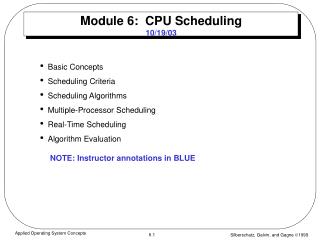
Module 6: CPU Scheduling 10/19/03. Basic Concepts Scheduling Criteria Scheduling Algorithms Multiple-Processor Scheduling Real-Time Scheduling Algorithm Evaluation NOTE: Instructor annotations in BLUE. Basic Concepts. Objective: Maximum CPU utilization obtained with multiprogramming

E N D
Module 6: CPU Scheduling10/19/03 • Basic Concepts • Scheduling Criteria • Scheduling Algorithms • Multiple-Processor Scheduling • Real-Time Scheduling • Algorithm EvaluationNOTE: Instructor annotations in BLUE Applied Operating System Concepts
Basic Concepts • Objective: Maximum CPU utilization obtained with multiprogramming • A process is executed util it must wait - typically for completion if I/O request, or a time quanta expires. • CPU–I/O Burst Cycle – Process execution consists of a cycle of CPU execution and I/O wait. • CPU burst distribution Applied Operating System Concepts
Alternating Sequence of CPU And I/O Bursts Applied Operating System Concepts
Histogram of CPU-burst Times “Tune” the scheduler to these statistics Applied Operating System Concepts
CPU Scheduler • Selects from among the processes in memory that are ready to execute, and allocates the CPU to one of them. • CPU scheduling decisions may take place when a process: 1. Runs until it Switches from running to waiting state … stop executing only when a needed resource or service is currently unavailable. 2. Switches from running to ready state in the middle of a burst – can stop execution at any time 3. Switches from waiting to ready. … ? 4. Runs until it Terminates. • Scheduling under 1 and 4 is nonpreemptive. • All other scheduling is preemptive. • Under nonpremptive scheduling, once a CPU is assigned to a process, the process keeps the CPU until it releases the CPU either by terminating or switching to wait state - “naturally” stop execution. Applied Operating System Concepts
Dispatcher • Dispatcher module gives control of the CPU to the process selected by the short-term scheduler; this involves: • switching context • switching to user mode • jumping to the proper location in the user program to restart that program • Dispatch latency – time it takes for the dispatcher to stop one process and start another running. • Both scheduler and dispatcher are performance “bottlenecks” in the OS, and must be made as fast and efficient as possible. Applied Operating System Concepts
Scheduling Criteria • CPU utilization – keep the CPU as busy as possible • Throughput – # of processes that complete their execution per time unit • Turnaround time – amount of time to execute a particular processOr: the time from time of submission to time of completion – includes waits in queues in addition to execute time. • Waiting time – amount of time a process has been waiting in the ready queue – sum of the times in ready queue - this is from the point of view scheduler - scheduler does not look at CPU time or I/O wait time (only ready queue time) if it minimizes “waiting time”. .. Get a process through the ready queue as soon as possible. • Response time – amount of time it takes from when a request was submitted until the first response is produced, not output (for time-sharing environment) Applied Operating System Concepts
Optimization Criteria • Max CPU utilization • Max throughput • Min turnaround time • Min waiting time • Min response time Applied Operating System Concepts
P1 P2 P3 0 24 27 30 First-Come, First-Served (FCFS) Scheduling • Example: ProcessBurst Time P1 24 P2 3 P3 3 • Suppose that the processes arrive in the order: P1 , P2 , P3The Gantt Chart for the schedule is: • Waiting time for P1 = 0; P2 = 24; P3 = 27 • Average waiting time: (0 + 24 + 27)/3 = 17 Applied Operating System Concepts
FCFS Scheduling (Cont.) Suppose that the processes arrive in the order P2 , P3 , P1 . • The Gantt chart for the schedule is: • Waiting time for P1 = 6;P2 = 0; P3 = 3 • Average waiting time: (6 + 0 + 3)/3 = 3 • Much better than previous case. • Convoy effect short process behind long process P2 P3 P1 0 3 6 30 Applied Operating System Concepts
Shortest-Job-First (SJF) Scheduling • Associate with each process the length of its next CPU burst. Use these lengths to schedule the process with the shortest time. • Two schemes: • nonpreemptive – once CPU given to the process it cannot be preempted until completes its CPU burst. • Preemptive – if a new process arrives with CPU burst length less than remaining time of current executing process, preempt. This scheme is know as the Shortest-Remaining-Time-First (SRTF). • SJF is optimal – gives minimum average waiting time for a given set of processes. Applied Operating System Concepts
Example of Non-Preemptive SJF Process Arrival TimeBurst Time P1 0.0 7 P2 2.0 4 P3 4.0 1 P4 5.0 4 • SJF (non-preemptive) • FCFS is “tie breaker” if burst times the same. • Average waiting time = (0 + 6 + 3 + 7)/4 - 4 P1 P3 P2 P4 0 3 7 8 12 16 Applied Operating System Concepts
Example of Preemptive SJF(Also called Shortest-Remaining-Time-First (SRTF) ) In order for a new arrival to preempt, its burst must be strictly less than current remaining time Process Arrival TimeBurst Time P1 0.0 7 P2 2.0 4 P3 4.0 1 P4 5.0 4 • SJF (preemptive) • Average waiting time = (9 + 1 + 0 +2)/4 = 3 P1 P2 P3 P2 P4 P1 11 16 0 2 4 5 7 Applied Operating System Concepts
Determining Length of Next CPU Burst • Can only estimate the length. • Can be done by using the length of previous CPU bursts, using exponential averaging. n+1 = tn + (1- )n n stores past history tn is “recent history is a weighting factor … recursive in n Applied Operating System Concepts
Examples of Exponential Averaging • =0 • n+1 = n • Recent history does not count. • =1 • n+1 = tn • Only the actual last CPU burst counts. • If we expand the formula, we get: n+1 = tn+(1 - ) tn -1 + … +(1 - )j tn -1 + … +(1 - )n=1 tn 0 • Since both and (1 - ) are less than or equal to 1, each successive term has less weight than its predecessor. Applied Operating System Concepts
Priority Scheduling • A priority number (integer) is associated with each process • The CPU is allocated to the process with the highest priority (smallest integer highest priority). • Preemptive • nonpreemptive • SJF is a priority scheduling where priority is the predicted next CPU burst time. • Problem: Starvation – low priority processes may never execute. • Solution: Aging – as time progresses increase the priority of the process - a “reward” for waiting in line a long time - let the old geezers move ahead! Applied Operating System Concepts
Round Robin (RR) • Each process gets a small unit of CPU time (time quantum), usually 10-100 milliseconds. After this time has elapsed, the process is preempted and added to the end of the ready queue • RR is a preemptive algorithm. • If there are n processes in the ready queue and the time quantum is q, then each process gets 1/n of the CPU time in chunks of at most q time units at once. No process waits more than (n-1)q time units. • Performance • q large FIFO • q small q must be large with respect to context switch, otherwise overhead is too high. ==> “processor sharing” - user thinks it has its own processor running at 1/n speed (n processors) Applied Operating System Concepts
P1 P2 P3 P4 P1 P3 P4 P1 P3 P3 Example: RR with Time Quantum = 20 FCFS is tie breaker Assume all arrive at 0 time in the order given. ProcessBurst Time P1 53 P2 17 P3 68 P4 24 • The Gantt chart is: • Typically, higher average turnaround than SJF, but better response. 0 20 37 57 77 97 117 121 134 154 162 Applied Operating System Concepts
How a Smaller Time Quantum Increases Context Switches Context switch overhead very critical for 3rd case - since overhead is independent of quanta time Applied Operating System Concepts
Turnaround Time Varies With The Time Quantum No strict correlation of TAT and time quanta size - except for below TAT can be improved if most processes finish each burst in one quanta EX: if 3 processes each have burst of 10, then for q = 1, avg_TAT = 29, but for q = burst = 10, avg_TAT = 20. ==> design tip: tune quanta to average burst. Applied Operating System Concepts
Multilevel Queue (no Feedback - see later) • Ready queue is partitioned into separate queues:foreground queue (interactive)background queue (batch) • Each queue has its own scheduling algorithm, foreground queue – RRbackground queue – FCFS • Scheduling must be done between the queues. • Fixed priority scheduling; i.e., serve all from foreground then from background. All higher priority queues must be empty before given queue is processed. Possibility of starvation. Assigned queue is for life of the process. • Time slice between queues – each queue gets a certain amount of CPU time which it can schedule amongst its processes; i.e.,80% to foreground in RR • 20% to background in FCFS Applied Operating System Concepts
Multilevel Queue Scheduling Applied Operating System Concepts
Multilevel Feedback Queue • A process can move between the various queues; aging can be implemented this way. • Multilevel-feedback-queue scheduler defined by the following parameters: • number of queues • scheduling algorithms for each queue • method used to determine when to upgrade a process • method used to determine when to demote a process • method used to determine which queue a process will enter when that process needs service Applied Operating System Concepts
Multilevel Feedback Queues Queue 0 - High priority Queue 1 Queue 2 Low priority Higher priority queues pre-empt lower priority queues on new arrivals Fig 6.7 Applied Operating System Concepts
Example of Multilevel Feedback Queue • Three queues: • Q0 – time quantum 8 milliseconds • Q1 – time quantum 16 milliseconds • Q2 – FCFS • Q2 longest jobs, with lowest priority, Q1 shortest jobs with highest priority. • Scheduling • A new job enters queue Q0which is served FCFS. When it gains CPU, job receives 8 milliseconds. If it does not finish in 8 milliseconds, job is moved to queue Q1(demoted). • At Q1 job is again served FCFS and receives 16 additional milliseconds. If it still does not complete, it is preempted and moved to queue Q2. • Again, Qn is not served until Qn-1 empty Applied Operating System Concepts
Multiple-Processor Scheduling • CPU scheduling more complex when multiple CPUs are available. • Homogeneous processors within a multiprocessor. • Load sharing • Symmetric Multiprocessing (SMP) – each processor makes its own scheduling decisions. • Asymmetric multiprocessing – only one processor accesses the system data structures, alleviating the need for data sharing. Applied Operating System Concepts
Real-Time Scheduling • Hard real-time systems – required to complete a critical task within a guaranteed amount of time. • Soft real-time computing – requires that critical processes receive priority over less fortunate ones. • Deadline scheduling used. Applied Operating System Concepts
Dispatch Latency Applied Operating System Concepts
Solaris 2 Thread Scheduling • 3 scheduling priority classes • Timesharing/interactive – lowest – for users • Within this class: Multilevel feedback queues longer time slices in lower priority queues • System – for kernel processes • Real time – Highest • Local Scheduling – How the threads library decides which thread to put onto an available LWP. Remember threads are time multiplexed on LWP’s • Global Scheduling – How the kernel decides which kernel thread to run next. • The local schedules for each class are “globalized” from the scheduler's point of view – all classes included. • LPW’s scheduled by kernel Applied Operating System Concepts
Solaris 2 Scheduling Only a few in this class Real time Fig. 6.10 Reserved for kernel use. Ex: Scheduler & paging daemon User processes Go here Applied Operating System Concepts
Java Thread Scheduling • JVM Uses a Preemptive, Priority-Based Scheduling Algorithm. • FIFO Queue is Used if There Are Multiple Threads With the Same Priority. Applied Operating System Concepts
Java Thread Scheduling (cont)-omit JVM Schedules a Thread to Run When: • The Currently Running Thread Exits the Runnable State. • A Higher Priority Thread Enters the Runnable State * Note – the JVM Does Not Specify Whether Threads are Time-Sliced or Not. Applied Operating System Concepts
Time-Slicing (Java) -omit • Since the JVM Doesn’t Ensure Time-Slicing, the yield() Method May Be Used: while (true) { // perform CPU-intensive task . . . Thread.yield(); } This Yields Control to Another Thread of Equal Priority. • Cooperative multi-tasking possible using yield Applied Operating System Concepts
Java Thread Priorities -omit • Thread Priorities:PriorityComment Thread.MIN_PRIORITY Minimum Thread Priority Thread.MAX_PRIORITY Maximum Thread Priority Thread.NORM_PRIORITY Default Thread Priority Priorities May Be Set Using setPriority() method: setPriority(Thread.NORM_PRIORITY + 2); Applied Operating System Concepts
Algorithm Evaluation • Deterministic modeling – takes a particular predetermined workload and defines the performance of each algorithm for that workload - what we’ve been doing in the examples - optimize various criteria. • Easy, but success depends on accuracy of input • Queuing models - statistical - need field measurements of statistics in various compouting environments • Implementation - Costly - OK is a lot of pre-implementation done first. Applied Operating System Concepts
Evaluation of CPU Schedulers by Simulation -need good models- drive it with field data and/orstatistical data - could be slow. Applied Operating System Concepts