Download
1 / 26
260 likes | 277 Views
Enhance decision-making with our Portfolio Analyzer, explore risk and stationarity principles, and examine real-world examples.

E N D
Portfolio Analyzer and Risk Stationarity Lecture 23 • Read Chapters 13 and 14 • Lecture 23 Portfolio Analyzer Example.xlsx • Lecture 23 Portfolio Analyzer 2015.XLSX • Lecture 23 Portfolio Low Correlation.XLSX • Lecture 23 Portfolio High Correlation.XLSX • Lecture 23 Changing Risk Over Time.XLSX • Lecture 23 CV Stationarity.XLSX
Portfolio and Bid Analysis Models • Many business decisions can be couched in a portfolio analysis framework • A portfolio analysis refers to comparing investment alternatives • A portfolio can represent any set of risky alternatives the decision maker considers • For example an insurance purchase decision can be framed as a portfolio analysis if many alternative insurance coverage levels are being considered
Portfolio Analysis Models • Basis for portfolio analysis – overall risk can be reduced by investing in two risky instruments rather than one IF: • This always holds true if the correlation between the risky investments is negative • Markowitz discovered this result 50+ years ago while he was a graduate student! • Old saw: “Don’t put all of your eggs in one basket” is the foundation for portfolio analysis
Portfolio Analysis Models • Application to business – given two enterprises with negative correlation on net returns, then we want a combination of the two rather than specializing in either one • Mid West used to raise corn and feed cattle, now raice corn and soybeans • Irrigated west grew cotton and alfalfa • Undiversified portfolio is grow only corn • Thousands of investments, which ones to include in the portfolio is the question? • Own stocks in IBM and Microsoft • Or GMC, Intel, and Cingular • Each is a portfolio, which is best?
Portfolio Analysis Models • Portfolio analysis with three stocks or investments • Find the best combination of the three • Note Corr Coef.
Portfolio Analysis Models • Nine portfolios analyzed, expressed as percentage combinations of Investments 1-3
Portfolio Analysis Models • The statistics for 9 simulated portfolios show variance reduction relative to investing exclusively in one instrument • Look at the CVs across Portfolios P1-P9, it is minimized with portfolio P7
Portfolio Analysis Models • Preferred is 100% invested in Invest 1 • Next best thing is P6, then P5
Portfolio Analysis Models • Next how does the preferred portfolio change as the investor considers investments with low correlation
Portfolio Analysis Models • The results for simulating 9 portfolios where the individual investments have low correlation and near equal means • Portfolios still have lower relative risk
Portfolio Analysis Models • A portfolio (P6) is ranked second followed by P5
Portfolio Analysis Models • How are portfolios observed in the investment world? • The following is a portfolio mix recommendation prepared by a major brokerage firm • The words are changed but see if you can find the portfolio for extremely risk averse and slightly risk averse investors
Portfolio Analysis Models • Simulation does not tell you the best portfolio, but tells you the rankings of alternative portfolios • Steps to follow for portfolio analysis • Select investments to analyze • Gather returns data for period of interest – annual, monthly, etc. based on frequency of changes • Simulate stochastic returns for investment i (or Ỹi) • Multiply returns by portfolio j fractions or Rij= Fj * Ỹi • Sum returns across investments for portfolio j or Pj = ∑ Rij sum across i investments for portfolio j • Simulate on the total returns (Pj) for all j portfolios • SERF ranking of distributions for total returns (Pj)
Portfolio Analysis Models • Typical portfolio analysis might look like: • Assume 10 investments so stochastic returns are Ỹi for i=1,10 • Assume two portfolios j=1,2 • Calculate weighted returns Rij = Ỹi * Fij where Fij is fraction of funds invested in investment i for portfolio j • Calculate total return for each j portfolio as Pj = ∑ Rij
Data for a Portfolio Analysis Models • Gather the prices of the stocks for the time period relevant to frequency of your investment decision • Monthly data if adjust portfolio monthly, etc. • Annual returns if adjust once a year • Convert the prices to percentage changes • Rt = (Pricet – Pricet-1) / Pricet-1 • Temptation is to use the prices directly rather than percentage returns • Brokerage houses provide prices on web in downloadable format to Excel
Covariance Stationary & Heteroskedasticy • Part of validation is to test if the standard deviation for random variables match the historical std dev. • Referred to as “covariance stationary” • Simulating outside the historical range causes a problem in that the mean will likely be different from history causing the coefficient of variation, CVSim, to differ from historical CVHist: CVHist= σH / ῩH Not Equal CVSim = σH / ῩS
Covariance Stationary • CV stationarity is likely a problem when simulating outside the sample period: • If Mean for X increases, CV declines, which implies less relative risk about the mean as time progresses CVSim = σH / ῩS • If Mean for X decreases, CV increases, which implies more relative risk about the mean as we get farther out with the forecast CVSim = σH / ῩS • See Chapter 9
CV Stationarity • The Normal distribution is covariance stationary BUT it is not CV stationary if the mean differs from historical mean • For example: • Historical Mean of 2.74 and Historical Std Dev of 1.84 • Assume the deterministic forecast for mean increases over time as: 2.73, 3.00, 3.25, 4.00, 4.50, and 5.00 • CV decreases while the std dev is constant
CV Stationarity for Normal Distribution • An adjustment to the StdDev can make the simulation results CV stationary if you are simulating a Normal dist. • Calculate a Jt+i value for each period (t+i) to simulate as: Jt+i= Ῡt+i / Ῡhistory • The Jt+i value is then used to simulate the random variable in period t+i as: Ỹt+i = Ῡt+i + (StdDevhistory * Jt+i * SND) Ỹt+i = NORM(Ῡt+i, StdDev * Jt+i) • The resulting random values for all years t+i have the same CV but different StdDev than the historical data • This is the result desired when doing multiple year simulations
CV Stationarity and Empirical Distribution • Empirical distribution automatically adjusts so the simulated values are CV stationary if the distribution is expressed as deviations from the mean or trend Ỹt+i = Ῡt+i * [1 + Empirical(Sj, F(Sj), USD)]
Empirical Distribution Validation • Empirical distribution as a fraction of trend or mean automatically adjusts so the simulated values are CV stationary • This poses a problem for validation • The correct method for validating Empirical distribution is: • Calculate the Mean and Std Dev to test against as follows • Mean = Historical mean * J • Std Dev = Historical mean * J * CV for simulated values / 100 • Here is an example for J = 2.0
Add Heteroskedasticy to Simulation • Sometimes we want the CV to change over time • Change in policy could increase the relative risk • Change in management strategy could change relative risk • Change in technology can change relative risk • Change in market volatility can change relative risk • Create an Expansion factor or Et+i value for each year to simulate • Et+i is a fractional adjustment to the relative risk • Here are the rules for setting and Expansion Factor • 0.0 results in No risk at all for the random variable • 1.0 results in same relative risk (CV) as the historical period • 1.5 results in 50% larger CV than historical period • 2.0 results in 100% larger CV than historical period • Chapter 9
Add Heteroskedasticy to Simulation • Simulate 5 years with no risk for the first year, historical risk in year 2, 15% greater risk in year 3, and 25% greater CV in years 4-5 • The Et+ivalues for years 1-5 are, respectively, 0.0, 1.0, 1.15, 1.25, 1.25 • Apply the Et+i expansion factors as follows: • Normal distribution Ỹt+i = Ῡt+i + (Std Devhistory * Jt+i* Et+i* SND)Ỹt+i=NORM (Ῡt+i, StdDevhistory * Jt+i* Et+i) • Empirical Distribution if Si are deviations from mean Ỹt+i = Ῡt+i * { 1 + [Empirical(Sj, F(Sj), USD) * Et+I]}