Technical Efficiency and Economic Efficiency
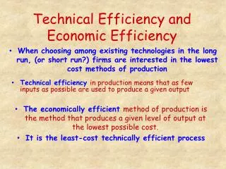
Technical Efficiency and Economic Efficiency. Technical efficiency in production means that as few inputs as possible are used to produce a given output. When choosing among existing technologies in the long run, (or short run?) firms are interested in the lowest cost methods of production.

Technical Efficiency and Economic Efficiency
E N D
Presentation Transcript
Technical Efficiency and Economic Efficiency • Technical efficiency in production means that as few inputs as possible are used to produce a given output • When choosing among existing technologies in the long run, (or short run?) firms are interested in the lowest cost methods of production • The economically efficient method of production is the method that produces a given level of output at the lowest possible cost. • It is the least-cost technically efficient process
Long Run Costs Economies of Scale More efficient as size increases Diseconomies of Scale Less efficient as size increases Constant Returns to Scale Efficient Range of Production
A Typical Long-Run Average Total Cost Table ATC falls because of economies of scale ATC is constant because of constant returns to scale ATC rises because of diseconomies of scale
A Typical Long-Run Average Total Cost Curve Costs per unit $60 Long-run average total cost (LRATC) Minimum efficient level of production $55 $50 Q 11 14 17 20 ATC falls because of economies of scale ATC rises because of diseconomies of scale ATC is constant because of constant returns to scale
Economies of Scale long-run average total costs decrease as output increases • Indivisible setup cost is the cost of an input for which a certain minimum amount of production must be undertaken before the input becomes economically feasible to use • Indivisible setup costs create many real-world economies of scale • The cost of a blast furnace or an oil refinery is an example of an indivisible setup cost
Theminimum efficient level of production is the amount of production that spreads setup costs out sufficiently for firms to undertake production profitably • reached once the size of the market expands to a size large enough for firms to take advantage of all economies of scale $60 Minimum efficient level of production $55 $50 Q 11 14 17 20
Constant Returns to Scale • the flat portion of the curve • when average total costs do not change as output increases • when production techniques can be replicated again and again to increase output • before monitoring costs rise and team spirit is lost
Diseconomies of Scale • when long-run average total costs increase as output increases • Usually, but not always, start occurring as firms get large • These are shown by the upward sloping portion of the long-run average total cost curve
Two reasons for diseconomies of scale are: • Increased monitoring costs (the costs incurred by the organizer of production in seeing to it that the employees do what they’re supposed to do) • Loss of team spirit (the feelings of friendship and being part of a team that bring out people’s best efforts)
Long-Run Average Total Cost Gets more efficient as size increases Gets less efficient as size increases Efficient Range of Production LRAC 60,000 Economies of Scale Diseconomies of Scale 50,000 40,000 30,000 20,000 Constant Returns to Scale 10,000 0 6 7 8 9 10 3 4 5 1 2 Hundred thousand Cars
Which of the following is most likely to be an implicit cost of production? • property taxes on a building owned by the firm • transportation costs paid to a trucking supplier • c. rental payments for a building utilized by the company and rented from another party • d. interest income foregone on funds invested in the firm by the owners 2. The law of diminishing returns a. explains why marginal cost eventually increases as output expands. b. implies that average fixed cost will remain unchanged as output expands. c. is true for physical production activities but not for activities such as studying. d. applies to a capitalist economy but would be irrelevant if the means of production were owned by the state. 3. Which of the following represents a long-run adjustment? a. the hiring of four additional cashiers by a supermarket b. a cutback on purchases of coke and iron ore by a steel manufacturer c. construction of a new assembly-line plant by a car manufacturer d. the extra dose of fertilizer used by a farmer on his wheat crop
4. The short-run average total cost (ATC) curve of a firm is U-shaped because a. larger firms always have lower per-unit costs than smaller firms. b. at low levels of output, AFC will be high, while at high levels of output, MC will be high as the result of diminishing returns. c. diminishing returns will be present when output is small, and high AFC will push per-unit cost to high levels when output is large. d. diseconomies of scale will be present at both small and large output rates. 5. When costs that vary with the level of output are divided by the output, you have calculated a. total changing cost. b. total fixed cost. c. average fixed cost. d. average variable cost. 6. A downward-sloping portion of a LR average total cost curve is the result of a. economies of scale. b. diseconomies of scale. c. diminishing returns. d. the existence of fixed resources. 7. In the short run, if average variable cost equals $50, average total cost equals $75, and output equals 100, the total fixed cost must be a. $25. b. $2,500. c. $5,000. d. $7,500.
At what output in the graph would the firm’s per-unit cost of production be minimized? • 3 b. 4 c. 5 d. 6 b. 4 • What is the firm’s approximate total cost when it produces three units? • 10 b. 16 c. 48 d. 60 c. 48 • What is the firm’s total cost when it produces four units? • 11 b. 15 c. 60 d. 75 c. 60 The average variable cost and average total cost for a firm are indicated in the graph. If the marginal cost curve were constructed, at what output would it cross the AVC curve? b. 15 • 10 b. 15 c. 20 d. 25 At what output should a the marginal cost curve cross the ATC curve? • 15 b. 20 c. 25 d. 30 b. 20