Download
1 / 50
720 likes | 1.41k Views
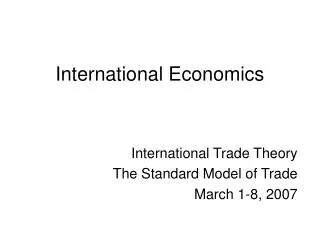
International Economics. Li Yumei Economics & Management School of Southwest University. International Economics. Chapter 3 The Standard Theory of International Trade. Organization. 3.1 Introduction 3.2 The Production Frontier with Increasing Costs 3.3 Community Indifference Curves

E N D
International Economics Li Yumei Economics & Management School of Southwest University
International Economics Chapter 3 The Standard Theory of International Trade
Organization • 3.1 Introduction • 3.2 The Production Frontier with Increasing Costs • 3.3 Community Indifference Curves • 3.4 Equilibrium in Isolation • 3.5 The Basis for and the Gains from Trade with Increasing Costs • 3.6 Trade Based on Differences in Tastes • Chapter Summary • Exercises
3.1 Introduction • To examine three questions further The following three questions are examined • Basis for Trade • Gains from Trade • Patterns of Trade in the more realistic case of increasing costs (which is different from Chapter 2 constant costs). • To introduce demand preferences or tastes (demand conditions) to extend the simple model (supply conditions)
3.2 The Production Frontier with Increasing Costs • Illustration of Increasing Costs • The Marginal Rate of Transformation • Reasons for Increasing Opportunity Costs and Different Production Frontiers • Comments • Conclusion
Illustration of Increasing Costs • Increasing Opportunity Costs Increasing opportunity costs mean that the nation must give up more and more of one commodity to release enough resources to produce each additional unit of another commodity. Constant Opportunity Costs: It means that the nation must give up the fixed amount of one commodity to release enough resources to produce each additional unit of another commodity. Decreasing Opportunity Costs: ?
Illustration of Increasing Costs • Illustration of Increasing Costs With increasing costs, each nation’s PPF (production possibility frontier) is concave (凹的) from the origin (rather than a straight line with constant costs). How to show the PPF in each nation with increasing Costs?
PPF (straight line) with Constant Costs FIGURE 2-1 The Production Possibility Frontiers of the United States and the United Kingdom with constant costs
Illustration of Increasing Costs FIGURE 3-1 Production Frontiers of Nation 1 and Nation 2 with Increasing Costs.
Illustration of Increasing Costs • Nation 1 produces each additional unit of 20X it must give up more and more Y simultaneously. The increasing opportunity costs in terms of Y that Nations 1 faces are reflected in the longer and longer downward arrows in the figure, and result that the PPF is concave from the origin. • Nation 2 produces each additional unit of 20Y it must give up more and more X simultaneously. The increasing opportunity costs in terms of X that Nation 2 faces are reflected in the longer and longer leftward arrows in the figure, and result that the PPF is concave from the origin. • Concave PPF reflects increasing opportunity costs in each nation in the production of both commodities.
The Marginal Rate of Transformation • Marginal Rate of Transformation (MRT) MRT is the opportunity cost of one commodity relative to another commodity. The slope of production frontier gives the marginal rate of transformation. E.G. See Figure 3-1 Nation 1(page 61) (1) MRT at point A ( ¼): It means that Nation 1 must give up ¼ of a unit of Y to release just enough resources to produce one additional unit of X at this point. (2) MRT at point B (1): It means that Nation 1 must give up one unit of Y to release just enough resources to produce one additional unit of X at this point. Reflecting the increasing opportunity costs.
Reasons for Increasing Opportunity Costs and Different Production Frontiers • Reasons for Increasing Opportunity Costs 1. Resources or factors of production are not homogeneous (e.g. all units of the same factor are not identical or of the same quality); 2. Resources or factors of production are not used in the same fixed proportion or intensity in the production of all commodities. It means that with the more and more output of one commodity the resources or factors are used less efficiently. Such as wheat land for milk production. (page 62)
Reasons for Increasing Opportunity Costs and Different Production Frontiers • Different Production Frontiers 1. Due to the fact that the two nations have different factor endowments or resources at their disposal (details in Chapter 5) and / or use different technologies in production. 2. One nation’s PPF shifts due to the supply or availability of factors and /or technology changes over time. And the type and extent of these shifts depend on the type and extent of the changes that take place (details in Chapter 7)
Comments • Even though the comparative advantage simple model extends to the more realistic case of increasing opportunity costs, it doesn’t explain the reasons that why different countries have different production possibility frontiers. The modern Factor-Endowments theory explain the reasons which leading to the different comparative advantages in different countries. • Only considering the supply factor with available technology to show the production possibility frontier to determine each nation’s comparative advantage. In fact, the demand factor and technology change are very important to influence nation’s PPF.
Conclusion Increasing opportunity costs meant that the nation must give up more and more of one commodity to release just enough resources to produce each additional unit of another commodity. This is reflected in a production frontier that is concave from the origin. The slope of the production frontier gives the marginal rate of transformation (MRT). Increasing opportunity costs arise because resources are not homogeneous and are not used in the same fixed proportion in the production of all commodities. Production frontiers differ because of different factor endowments and /or technology in different nations.
3.3 Community Indifference Curves • Illustration of Community Indifference Curves • The Marginal Rate of Substitution • Some Difficulties with Community Indifference Curves • Comments • Conclusion
Illustration of Community Indifference Curves • Community Indifference Curves 1. They reflect the demand preferences or the tastes in a nation. 2. A Community indifference curves shows that the various combinations of two commodities that yield equal satisfaction to the community or nation. 3. Higher curves refer to greater satisfaction, lower curves to less satisfaction. 4. Community indifference curves are negatively sloped and convex from the origin.
Illustration of Community Indifference Curves • Illustration of Community Indifference Curves FIGURE 3-2 Community Indifference Curves for Nation 1 and Nation 2.
Illustration of Community Indifference Curves • Explanation of Figure 3.2 1. Higher indifference curves higher satisfaction Points N and A give equal satisfaction to Nation 1, since they are both on indifference curve Ⅰ. Points T and H refer to a higher level of satisfaction, since they are on a higher indifference curve Ⅱ. Point E refers to greater satisfaction, since it is on the indifference curve Ⅲ. ( N=A ﹤T,H ﹤E) . In Nation 2, A’=R’ ﹤H’﹤E’. 2. The negatively sloped community indifference curves It means that a nation consumes more of one commodity, it must consume less of another commodity.
The Marginal Rate of Substitution • Marginal Rate of Substitution (MRS) 1. MRS of one commodity for another commodity in consumption refers to the amount of another commodity that a nation could give up for one extra unit of one commodity and still remain on the same indifference curve. 2. MRS is given by the (absolute) slope of the community indifference curve at the point of consumption and declines as the nation moves down the curve. (See page 63 Figure 3.2: in Nation 1 MRS of X at point N is greater than point A; in Nation 2 MRS of X of point A’ is greater than point R’)
The Marginal Rate of Substitution • Marginal Rate of Substitution (MRS) 3. The decline in MRS or absolute slope of an indifference curve is a reflection of the fact that the more of X and the less of Y a nation consumes, the more valuable to the nation is a unit of Y at the margin compared with a unit of X. Therefore, the nation can give up less and less of Y for each additional unit of X it wants. 4. Declining MRS means that community indifference curves are convex from the origin. Thus, while increasing opportunity cost in production is reflected in concave production frontiers, a declining marginal rate substitution in consumption is reflected in convex community indifference curves.
Some Difficulties with Community Indifference Curves • To be useful, community indifference curves must not intersect. Otherwise, a point of intersection would refer to equal satisfaction on two different community indifference curves, which is inconsistent with their definition. • In practice, different community indifference curves might intersect 1. Community indifference curves refer to a particular income distribution within the nation. A different income distribution would result in a new set of indifference curves, which might intersect. 2. Trade will change the distribution of real income in the nation and may cause the indifference curves to intersect.
Some Difficulties with Community Indifference Curves • Solution of the impasse Compensation principle: 1. Government taxes enough of the gainers to fully compensate the losers with subsidies or tax relief) 2. Restriction assumptions about tastes, incomes and patterns of consumption to preclude intersecting community indifference curves Here the compensation principle or restrictive assumptions do not completely eliminate all the conceptual difficulties inherent in using community indifference curves. We still draw them as nonintersecting
Comments • Community Indifference Curves The demand factor is introduced into the simple trade model, and it makes the model more realistic. • Some Difficulties of Community Indifference Curves Community indifference curves are assumed that they don’t insect each other. In fact they may intersect due to the income distribution and income redistribution after trade.
Conclusion A community indifference curve shows the various combinations of two commodities that yield equal satisfaction to the community or nation. Higher curves refer to a greater level of satisfaction. Community indifference curves are negatively sloped and convex from the origin. And to be useful, they must not cross. The slope of an indifference curve gives the marginal rate of substitution (MRS) in consumption, or the amount of commodity Y that a nation could give up for each extra unit of commodity X and still remain on the same indifference curve. Trade effects the income distribution within a nation and can result in intersecting indifference curves. This difficulty can be overcome by the compensation principle, which states that the nation gains from trade if the gainers would retain some of their gain even after fully compensating losers for their losses. Alternatively, some restrictive assumptions could be made.
3.4 Equilibrium in Isolation • Illustration of Equilibrium in Isolation • Equilibrium-Relative Commodity Prices and Comparative Advantage • Conclusion
Illustration of Equilibrium in Isolation • Introduction In section 3.2 the production or supply conditions (production possibility frontier) are discussed in a nation; In section 3.3 the tastes or demand preference conditions (community indifference curves) are discussed in a nation. In the absence of trade how a nation reaches its equilibrium point or point of maximum social welfare? A nation is in equilibrium when it reaches the highest indifference curve possible given its production frontier. That is to say, the point where its production frontier is tangent to indifference curve is the equilibrium point in a nation.
Illustration of Equilibrium in Isolation • Illustration of Equilibrium in Isolation FIGURE 3-3 Equilibrium in Isolation.
Equilibrium-Relative Commodity Prices and Comparative Advantage • Equilibrium-relative commodity price in isolation It is given by the slope of the common tangent to the nation’s production frontier and indifference curve at the autarky (in the absence of trade) point of production and Consumption. (see Figure 3.3 page 66) E.G. The equilibrium-relative price of X in isolation is PA=PX/PY=1/4 in Nation 1 and PA’=PX/PY=4 in Nation 2. Since PA﹤PA’, Nation 1 has a comparative advantage in commodity X and Nation 2 in commodity Y.
Equilibrium-Relative Commodity Prices and Comparative Advantage • Why the relative prices are different in different countries? Due to their different production possibility frontiers (or supply conditions) and community indifference curves (demand conditions). • How to determine one nation’s equilibrium point in isolation? The forces of supply (as given by the nation’s PPF) and the forces of demand (as summarized by the nation’s indifference curves or maps) together determine the equilibrium-relative commodity prices in each nation in autarky.
Case Study 3-1 Comparative advantage of the Unites States, the European Union and Japan • Revealed Comparative Advantage (显性比较优势) It refers to the excess in the percentage of total exports over the percentage of total imports in each major commodity group for each country or region. See page 67 table 3.1
Conclusion In the absence of trade, a nation is in equilibrium when it reaches the highest indifference curve possible with its production frontier. This occurs at the point where a community indifference curve is tangent to the nation’s production frontier. The common slope of the two curves at the tangency point gives the internal equilibrium-relative commodity price in the nation and reflects the nation’s comparative advantage.
3.5 The Basis for and the Gains from Trade with Increasing Costs • Illustrations of the Basis for and the Gains from Trade with Increasing Costs • Equilibrium-Relative Commodity Prices with Trade • Incomplete Specialization • Small-Country Case with Increasing Costs • The Gains from Exchange and from Specialization • Conclusion
Illustrations of the Basis for and the Gains from Trade with Increasing Costs • Relative-Commodity Prices A difference in relative commodity prices between two nations is a reflection of their comparative advantage and form the basis for mutually beneficial trade. Lower relative commodity prices mean the comparative advantage while higher relative commodity prices mean the comparative disadvantage. Each nation should then specialize in the production of the commodity of its comparative advantage and exchange par of its output with the other nation for the commodity of its comparative disadvantage.
Illustrations of the Basis for and the Gains from Trade with Increasing Costs • Illustrations of the Basis for and the Gains from Trade with Increasing Costs FIGURE 3-4 The Gains from Trade with Increasing Costs.
Illustrations of the Basis for and the Gains from Trade with Increasing Costs • Explanation of Figure 3.4 1. With increasing costs, the specialization will continue until relative commodity prices in the two nations become equal at the level at which trade is in equilibrium. PX/PY=1. By then trading with each other, both nations can benefit from the trade. Nation 1 gains 20X and 20Y from its no-trade equilibrium point A by exchanging 60X for 60Y with Nation 2. Nation 2 gains 20 X and 20Y from its no-trade equilibrium point A’ by exchanging 60Y for 60X with Nation 1. 2. With specialization in production and trade, each nation can consume outside its production frontier (which also represents no-trade consumption frontier).
Equilibrium-Relative Commodity Prices with Trade • Equilibrium-relative Commodity Price with Trade It is the common relative price in both nations at which trade is balanced. E.G. Figure 3.4 PB=PB’=1. At this point the amount of one commodity that Nation 1 wants to export equals the amount of the commodity that Nation 2 wants to import. Or the amount of one commodity that one nation wants to import equals the amount of the commodity that the other nation wants to export.
Incomplete Specialization • Incomplete Specialization This is the basic difference between the trade model under increasing costs and the constant costs. Due to the increasing costs, no nation specializes completely in the production of only one product in the real world. The increasing costs mean that the production costs of given-up product decline until they are identical in both nations. Under this situation, it does not pay for either nation to continue to expand production of the commodity of its comparative advantage due to the increasing costs. (Case study 3-2 page 71)
Small-Country Case with Increasing Costs • Small – Country Case 1. Under constant cost, the complete specialization happens in a small country while a large country continue to produce both commodities even with trade due to the dissatisfaction demand for the imports from a small country. 2. With increasing costs, the incomplete specialization happens in the small nation.
The Gains from Exchange and from Specialization • Gains from Trade The gains from trade can be broken down into two components: the gains from exchange and the gains from specialization. FIGURE 3-5 The Gains from Exchange and from Specialization.
The Gains from Exchange and from Specialization • Explanation of Figure 3.5 page 72 1. Gains from exchange: from A to T, Nation 1 exports 20X for 20Y at the prevailing world market price of PW=1 and end up consuming at point T. 2. Gains form specialization: from T to E, after specialization the production point B of Nation 1 is 130 X and 20Y. Nation 1 exchange 60X for 60Y and consumes at point E. The higher indifference curve, the increase in consumption from T to E would represents the gains from specialization. (Case study 3.3 and 3.4 page from 74 to 75)
Conclusion With trade, each nation specializes in producing the commodity of its comparative advantage and faces increasing opportunity costs. Specialization in production proceeds until relative commodity prices in the two nations are equalized at the level at which trade is in equilibrium. By the trading, each nation ends up consuming on a higher indifference curve than in the absence of trade. With increasing costs, specialization in production is incomplete, even in a small nation. The gains from trade can be broken down into gains from exchange and gains from specialization in production.
3.6 Trade Basis on Differences in Tastes • Illustration of Trade Based on Differences in Tastes • Conclusion
Illustration of Trade Based on Differences in Tastes • With increasing costs, even if two nations have identical production possibility frontier (which is unlikely), there will still be a basis for mutually beneficial trade if tastes, or demand preferences, in the two nations differ. • Illustration of Trade Based on Differences in Tastes
Illustration of Trade Based on Differences in Tastes • Explanation of Figure 3.6 1. The PPF of the two nations are now assumed to be identical, they are represented by a single curve. 2. The pretrade-relative price of X is lower in Nation 1 than in Nation 2. X is the comparative advantage of Nation 1 while Nation 2 is Y. 3. With the opening of trade, Nation 1 specializes in the production of X (and moves down its production frontier) while Nation 2 specializes in the production of Y (and moves up its own production frontier). Specialization continues until PX/PY is the same in both nations and trade is balanced.
Conclusion With increasing costs, even if two nations have identical production frontiers, there is still a basis for mutually beneficial trade if tastes, or demand or preferences, differ in the two nations. The nation with the relatively smaller demand or preference for a commodity will have a lower autarky-relative price for, and a comparative advantage in, that commodity. This will set the stage of specialization in production and mutually beneficial trade, as described earlier.
Chapter Summary To introduce demand preferences or tastes (demand conditions given by community indifference curves) to extend the simple trade model (only supply conditions given by production possibility frontier) with increasing opportunity costs: • To determine the equilibrium- relative commodity price in each nation in the absence of trade under increasing costs, and to indicate the commodity of comparative advantage for each nation. • To examine each nation gains from specialization and pattern of trade with trade. • Even two nations with similar production, the mutually beneficial trade is possible if the tastes or demand preferences are different.
Exercises For an exposition of the gains from trade, see: • P.A. Samuelson, “The Gains from International Trade,”, May 1939, pp. 195-205. • P.A. Samuelson, “ The Gains from International Trade Once Again,” Economic Journal, December 1962, pp. 820-829 The changing pattern of comparative advantage in the United States and other industrial nations is examined in: • B. Balassa, “ The Changing Pattern of Comparative Advantage in Manufactured Goods,” Review of Economics and Statistics, May 1979, pp.259-266 • R.D. Richardson and C.Zhang, Revealing Comparative Advantage, NBER Working Paper No. 7212, July 1999
Internet Materials • http://www.imf.org • http://www.wto.org • http://www.imf.org/external/pubs/ft/issues10 • http://www.imf.org/external/pubs/ft/wp/WP9742.PDF • http://www.worldbank.org • http://www.un.org/depts/unsd/mbsreg.htm