Download

1 / 36
360 likes | 495 Views
Decision Trees SLIQ – fast scalable classifier Group 12 -Vaibhav Chopda -Tarun Bahadur. Paper By - Manish Mehta, Rakesh Agarwal and Jorma Rissanen Source – http://citeseer.ifi.unizh.ch/mehta96sliq.html

E N D
Decision TreesSLIQ – fast scalable classifierGroup 12-Vaibhav Chopda-Tarun Bahadur
Paper By - Manish Mehta, Rakesh Agarwal and Jorma Rissanen • Source – http://citeseer.ifi.unizh.ch/mehta96sliq.html • Material Includes: lecture notes for CSE634 – Prof. Anita Wasilewska http://www.cs.sunysb.edu/~cse634
Agenda • What is classification … • Why decision trees ? • The ID3 algorithm • Limitations of ID3 algorithm • SLIQ – fast scalable classifier for DataMining • SPRINT – the successor of SLIQ
Training Data Classifier (Model) Classification Process : Model Construction Classification Algorithms IF rank = ‘professor’ OR years > 6 THEN tenured = ‘yes’ CSE634 course notes – Prof. Anita Wasilewska
Classifier Testing Data Unseen Data Testing and Prediction (by a classifier) (Jeff, Professor, 4) Tenured? CSE634 course notes – Prof. Anita Wasilewska
Classification by Decision Tree Induction • Decision tree(Tuples flow along the tree structure) • Internal node denotes an attribute • Branch represents the values of the node attribute • Leaf nodes represent class labels or class distribution CSE634 course notes – Prof. Anita Wasilewska
Classification by Decision Tree Induction • Decision tree generation consists of two phases • Tree construction • At start we choose one attribute as the root and put all its values as branches • We choose recursively internal nodes (attributes) with their proper values as branches. • We Stop when • all the samples (records) are of the same class, then the node becomes the leaf labeled with that class • or there is no more samples left • or there is no more new attributes to be put as the nodes. In this case we apply MAJORITY VOTING to classify the node. • Tree pruning • Identify and remove branches that reflect noise or outliers CSE634 course notes – Prof. Anita Wasilewska
Classification by Decision Tree Induction • Wheres the challenge ? • Good choice of root attribute • Good choice of the internal nodes attributes is a crucial point. • Decision Tree Induction Algorithms differ on methods of evaluating and choosing the root and internal nodes attributes. CSE634 course notes – Prof. Anita Wasilewska
Basic Idea of ID3/C4.5 Algorithm - greedy algorithm - constructs decision trees in a top-down recursive divide-and-conquer manner. • Tree STARTS as a single node (root) representing all training dataset (samples) • IF the samples are ALL in the same class, THEN the node becomes a LEAF and is labeled with that class • OTHERWISE, the algorithm uses an entropy-based measure known as information gain as a heuristic for selecting the ATTRIBUTE that will BEST separate the samples into individual classes. This attribute becomes the node-name (test, or tree split decision attribute) CSE634 course notes – Prof. Anita Wasilewska
Basic Idea of ID3/C4.5 Algorithm (2) • A branch is created for each value of the node-attribute (and is labeled by this value -this is syntax) and the samples are partitioned accordingly (this is semantics; see example which follows) • The algorithm uses the same process recursively to form a decision tree at each partition. Once an attribute has occurred at a node, it need not be considered in any other of the node’s descendents • The recursive partitioningSTOPS only when any one of the following conditions is true. • All records (samples) for the given node belong to the same class or • There are no remaining attributes on which the • Records (samples) may be further partitioning. In this case we convert the given node into a LEAF and label it with the class in majority among samples (majority voting) • There is no records (samples) left – a leaf is created with majority vote for training sample CSE634 course notes – Prof. Anita Wasilewska
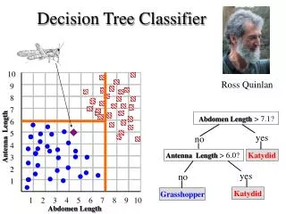
Example from professor Anita’s slide This follows an example from Quinlan’s ID3 CSE634 course notes – Prof. Anita Wasilewska
Shortcommings of ID3 • Scalability ? requires lot of computation at every stage of construction of decision tree • Scalability ? needs all the training data to be in the memory • It does not suggest any standard splitting index for range attributes
SLIQ - a decision tree classifier Features of SLIQ • Applies to both numerical and categorical attributes • Builds compact and accurate trees • Uses a pre-sorting technique in the tree growing phase and an inexpensive pruning algorithm • Suitable for classification of large disk-resident datasets, independently of the number of classes, attributes and records
SLIQ Methodology: Create decision tree by partitioning records Generate attribute list for each attribute Sort attribute lists for NUMERIC Attributes Start End
Attribute listing phase : Age – NUMERIC attribute CarType – CATEGORICAL attribute
Presorting Phase: Only NUMERIC attributes sorted CATEGORICAL attribute need not be sorted
Constructing the decision tree • (block 20) for each leaf node being examined, the method determines a split test to best separate the records at the examined node using the attribute lists in block 21. • (block 22) the records at the examined leaf node are partitioned according to the best split test at that node to form new leaf nodes, which are also child nodes of the examined node. • The records at each new leaf node are checked at block 23 to see if they are of the same class. If this condition has not been achieved, the splitting process is repeated starting with block 24 for each newly formed leaf node until each leaf node contains records from one class. In finding the best split test (or split point) at a leaf node, a splitting index corresponding to a criterion used for splitting the records may be used to help evaluate possible splits. This splitting index indicates how well the criterion separates the record classes. The splitting index is preferably a gini index.
Gini Index • The gini index is used to evaluate the “goodness” of the alternative splits for an attribute • If a data set T contains examples from n classes, gini(T) is defined as Where pj is the relative ferquency of class j in the data set T. • After splitting T into two subset T1 and T2 the gini index of the split data is defined as
Gini Index : The preferred splitting index • Advantage of the gini index: Its calculation requires only the distribution of the class values in each record partition. To find the best split point for a node, the node's attribute lists are scanned to evaluate the splits for the attributes. The attribute containing the split point with the lowest value for the gini index is used for splitting the node's records. • The following is the splitting test (next slide) – The flow chart will fit in the block 21 of decision tree construction
Determining subset of highest index Greedy algorithm may be used here The logic of finding best subset – substitute for block 39