Download
1 / 99
1.03k likes | 1.35k Views
Proper Univariate and Multivariate Integrals. Rajandra Chadra Bhowmik Lecturer Dept. of Mathematics Pabna Science and Technology University. Let’s start with some classical problems. What is the area of a circle?. How is it = pi*(radius) 2 ???. What is the volume of a sphere?.

E N D
Proper Univariate and Multivariate Integrals Rajandra Chadra Bhowmik Lecturer Dept. of Mathematics Pabna Science and Technology University
Let’s start with some classical problems • What is the area of a circle? How is it = pi*(radius)2 ??? • What is the volume of a sphere? How is it = 4*pi*radius3/3 ??? • What is the mass of a wire? • if density is given???
Lecture contents • Pre-history and Archimedes • Invention of Newton and Leibnitz • Definite integrals and Riemann • Geometric Interpretation and Applications of Definite Integrals • Double Integrals and Triple Integrals • Applications of Double Integrals and Triple Integrals • Line Integrals • Applications of Line Integrals
Pre-history and Archimedes • Integration can be traced as far back as ancient Egypt, circa 1800 BC, with the Moscow Mathematical Papyrus demonstrating knowledge of a formula for the volume of a pyramidal frustum. • The first documented systematic technique capable of determining integrals is the method of exhaustion of Eudoxus (circa 370 BC), which sought to find areas and volumes by breaking them up into an infinite number of shapes for which the area or volume was known. • This method was further developed and employed by Archimedes (287 BC - 212 BC) and used to calculate areas for parabolas and an approximation to the area of a circle. Archimedes devised a heuristic method based on statistics to do private calculations that would be classified today as integral calculus, but then presented rigorous geometric proofs for his results. To what extent Archimedes’ version of integral calculus was correct is debatable.
Invention of Newton and Leibnitz • The major advance in integration came in the 17th century with the independent discovery of the fundamental theorem of calculus by Newton(1642-1727)and Leibnitz(1646-1716). • The theorem demonstrates a connection between integration and differentiation. This connection, combined with the comparative ease of differentiation, can be exploited to calculate integrals. • In particular, the fundamental theorem of calculus allows one to solve a much broader class of problems. Equal in importance is the comprehensive mathematical framework that both Newton and Leibnitz developed. Given the name infinitesimal calculus, it allowed for precise analysis of functions within continuous domains. This framework eventually became modern calculus, whose notation for integrals is drawn directly from the work of Leibnitz.
Drawbacks of Newton and Leibnitz • While Newton and Leibnitz provided a systematic approach to integration, their work lacked a degree of rigor. • Bishop Berkeley memorably attacked infinitesimals as "the ghosts of departed quantities". • Calculus acquired a firmer footing with the development of limits and was given a suitable foundation by Cauchy in the first half of the 19th century.
Definition of Riemann integral • Let [a, b] be a compact (closed and bounded) interval in R. • Let p={a=x0,x1,x2,..,xn=b}, with xk-1<=xkfor k=1,2,…,n, be a partition of [a, b]. • Let f be a bounded real function defined on [a, b] • Integration was first rigorously formalized, using limits, by German MathematicianRiemann (1826-1866)
Graphical Representations f a=x0 x1 ξ2 x2 ξk xk ξn ξ1 Xk-1 Xn-1 Xn=b ∆xk ∆xn ∆x1 ∆x2
Definition of Riemann integral • Write ∆xk=xk-xk-1 for k = 1,2,…,n. • Set δ = max {∆xk : k = 1,2,…,n} • For each k = 1,2,…,n, Choose point • Then the Riemann integral of f with respect to x is defined by • Provided the limits exist.
Graphical Representations f(ξn)∆xn f(ξn) f(ξk)∆xk f f(ξ2)∆x2 f(ξk) f(ξ1)∆x1 f(ξ2) f(ξ1) x0=a x1 ξ2 x2 ξk xk ξn ξ1 Xk-1 Xn-1 Xn=b ∆xk ∆xn ∆x1 ∆x2
Riemann Integral(Rigorous definition ) • Let [a, b] be a compact (closed and bounded) interval in R. • Let p={a=x0,x1,x2,..,xn=b}, with xk-1<=xkfor k=1,2,…,n, be a partition of [a, b]. • Write ∆xk=xk-xk-1 for k = 1,2,…,n. • Let f be a bounded real function defined on [a, b]
Corresponding to each partition P, and k=1,2,…n,put And then
Lower sum L(P, f) mn ∆xn mk ∆xk f m2 ∆x2 m3 ∆x3 m1 ∆x1 xk x0=a x1 x2 x3 Xk-1 Xn-1 Xn=b ∆xk ∆xn ∆x1 ∆x2 ∆x3
Upper sum U(P, f) Mn ∆xn Mk ∆xk f M2 ∆x2 M3 ∆x3 M1 ∆x1 xk x0=a x1 x2 x3 Xk-1 Xn-1 Xn=b ∆xk ∆xn ∆x1 ∆x2 ∆x3
Let be the set of all partitions of [a, b]. Then, finally taking infimum and supremum over all partitions of [a, b] to define the upper Riemann integral and lower Riemann integralrespectively as
If the lower Riemann integral and the upper Riemann integral are equal, then we say that the function is Riemann integrable on [a, b] and write • In this case we write the integral as
It is called a dummy variable because the answer does not depend on the variable chosen. upper limit of integration Integration Symbol integrand variable of integration (dummy variable) lower limit of integration
The exact value from integration xk x0=a x1 x2 x3 Xk-1 Xn-1 Xn=b ∆xk ∆xn ∆x1 ∆x2 ∆x3
Some results • For every P, • For any refinement P*(a super set of P) of P,
<= M (b-a) M (b-a) f xk x0=a x1 x2 x3 Xk-1 Xn-1 Xn=b ∆xk ∆xn ∆x1 ∆x2 ∆x3
<= U (P1, f) <= M (b-a) M1 ∆x1 M2 ∆x2 f x0=a X1 X2=b ∆x1 ∆x2
<=U (P2, f)<= U (P1, f) <= M (b-a) M3 ∆x3 M1 ∆x1 f M2 ∆x2 x0=a X1 X2 X2=b ∆x1 ∆x2 ∆x3
m (b-a) <= f m (b-a) xk x0=a x1 x2 x3 Xk-1 Xn-1 Xn=b ∆xk ∆xn ∆x1 ∆x2 ∆x3
m (b-a)<= L (P1, f)<= f m2 ∆x2 m1 ∆x1 x0=a X1 X2=b ∆x1 ∆x2
m (b-a) <= L (P1, f) <=L (P2, f) <= m3 ∆x3 f m2 ∆x2 m1 ∆x1 x0=a X1 X2 X2=b ∆x1 ∆x2 ∆x3
Necessary and sufficient conditions • f is continuous on [a, b] implies f is Riemann integrable on [a, b]. • f is monotonic on [a, b] implies f is Riemann integrable on [a, b]. • f is bounded on [a, b] and f has only finitely many points of discontinuity on [a, b] implies f is Riemann integrable on [a, b]. • A bounded function f on a compact interval is integrable iff its set of discontinuities has measure zero(0). Proof of the Theorem is out of scope here (a matter of Lebesgue Integration in Measure Theory). For instant, we only say that all countable sets, including finite sets, and the Cantor set have measure 0, so that functions that are discontinuous only on these sets are integrable.
Dirichlet function and Thomae function Both functions are bounded. First one is discontinuous everywhere in R. i.e. the set of discontinuities has a nonzero measure. On the other hand, second one is discontinuous only at the rationals. i.e. set of discontinuities has measure 0. So, Dirichlet function is not integrable but Thomae function is.
Proof: • Let f be a real Riemann integrable function on [a, b]. Then for any arbitrary ε >0, we must have a partition P={a=x0, x1,x2,…,xn=b} with U(P, f)-L(P, f) < ε • Now for each k=1,2,….,n, applying Mean Value Theorem in the interval [xk-1, xk], we must have tk in [xk-1, xk] such that F(xk) - F(xk-1) = ∆xk F/(tk) = f(tk) ∆xk
Drawbacks of Riemann Integral • Although all bounded piecewise continuous functions are Riemann integrable on a bounded interval, subsequently more general functions were considered, to which Riemann's definition does not apply. • Stieltjeformulated an integral called Stietjes integral, to which Riemann integral is a special case. • Lebesgue formulated a different definition of integral, founded in measure theory (a subfield of real analysis). • Other definitions of integral, extending Riemann's and Lebesgue's approaches, were proposed.
Drawbacks of Riemann Integral • A major limitation towards more widespread implementation of Bayesian approaches is that obtaining the posterior distribution often requires the integration of high-dimensional functions. This can be computationally very difficult, among the several approaches short of direct integration Markov Chain Monte Carlo (MCMC) methods is one which attempt to simulate direct draws from some complex distribution of interest. • MCMC approaches are so-named because one uses the previous sample values to randomly generate the next sample value, generating a Markov chain (as the transition probabilities between sample values are only a function of the most recent sample value).
Drawbacks of Riemann Integral • Markov chain Monte Carlo integration, or MCMC, is a term used to cover a broad range of methods for numerically computing probabilities, or for optimization. They are simulation methods, mostly used in complex stochastic systems where exact computation and even simple simulation are not computationally feasible. • Methods that fall under this heading include Metropolis sampling, Hastings sampling and Gibbs sampling which are for integration and simulated annealing and sometimes genetic algorithms which are optimization techniques. • Although these methods are mainly used for complex systems it can be used to find the exact p-value for a test of association between the rows and columns of a contingency table.
Geometrical meaning of Definite Integrals • Let f be a realnon-negative continuous function defined in the closed interval [a, b]. Then
Area and Definite integral Curve y= f (x) Vertical linex=b R Vertical linex=a x0=a Xn=b X-axis
Geometrical meaning of Definite Integrals • Let f be a realcontinuous function (non negativity is not assured) defined in the closed interval [a, b]. Then
Area and Definite integral A1 R 1 f A2 x0=a Xn=b R 2 c
Applications of Definite Integrals (1) (Area of a region) Let f and g are continuous functions on the interval [a, b] with f (x) >= g (x) in [a, b]. Then the area A of the region • bounded above by the curve y = f (x) • below by the curve y = g (x) • between the vertical line x =a and x = b is given by
Area of the region Rbounded byy = sqrt (x) and y = x.^2(filled red)
Application of Definite Integrals (2)(Volume of solid revolution) • Theorem: Let S be a solid bounded by two parallel planes perpendicular to the x-axis at x = a and x = b[[ y-axis at y = c and y = d]], If, for each x in [a, b] [[y in [c, d] ]], the cross sectional area of S perpendicular to the x-axis is A (x) [[y-axis is B(y) ]], then the volume of the solid is
Solid Revolution • Let f be continuous and non negative in [a, b] and let R be the region bounded by y = f (x) above x-axis between x = a and x = b. Then the solid generated by revolving the region R about the x-axis is such as require in the above theorem [each cross sectional area is a circular disk with radius f (x)]. Thus volume of the solid revolution is
On the other hand, we know volume of a cone of radius r (=3/2) and height h (=3) is