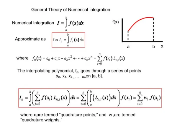
5.5 Numerical Integration

1. Photo by Vickie Kelly, 1998 Greg Kelly, Hanford High School, Richland, Washington 5.5 Numerical Integration Mt. Shasta, California

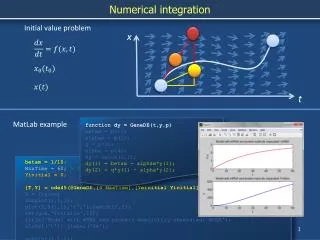
2. Using integrals to find area works extremely well as long as we can find the antiderivative of the function. Sometimes, the function is too complicated to find the antiderivative. At other times, we don’t even have a function, but only measurements taken from real life. What we need is an efficient method to estimate area when we can not find the antiderivative.

3. Actual area under curve:

4. Approximate area: Left-hand rectangular approximation: (too low)

5. Approximate area: Right-hand rectangular approximation: (too high)

6. Averaging the two: (too high) 1.25% error

7. Averaging right and left rectangles gives us trapezoids:

8. (still too high)

9. Trapezoidal Rule: ( h = width of subinterval ) This gives us a better approximation than either left or right rectangles.

10. Approximate area: Compare this with the Midpoint Rule: 0.625% error (too low) The midpoint rule gives a closer approximation than the trapezoidal rule, but in the opposite direction.

11. Trapezoidal Rule: (too high) 1.25% error Midpoint Rule: 0.625% error (too low) Ahhh! Oooh! Wow! Notice that the trapezoidal rule gives us an answer that has twice as much error as the midpoint rule, but in the opposite direction. If we use a weighted average: This is the exact answer!

12. twice midpoint trapezoidal This weighted approximation gives us a closer approximation than the midpoint or trapezoidal rules. Midpoint: Trapezoidal:

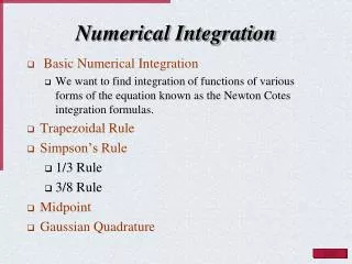
13. Simpson’s Rule: ( h = width of subinterval, n must be even ) Example:

14. Simpson’s rule can also be interpreted as fitting parabolas to sections of the curve, which is why this example came out exactly. Simpson’s rule will usually give a very good approximation with relatively few subintervals. It is especially useful when we have no equation and the data points are determined experimentally. p