Download
1 / 66
660 likes | 733 Views
Finance:- The Economics of allocating resources across time or reallocation of recourses in time , Such as borrowing and Lending money raising capital. Financial Investment:- Borrowing / Lending / Buying shares ……etc ( Needs provision of funds)

E N D
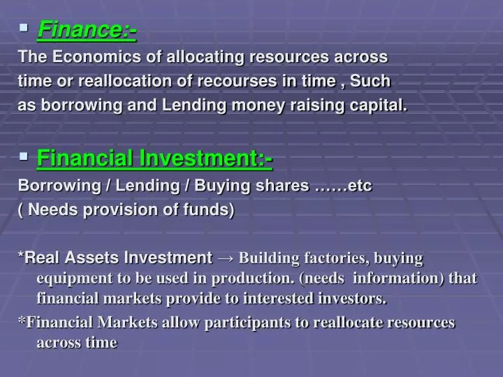
Finance:- The Economics of allocating resources across time or reallocation of recourses in time , Such as borrowing and Lending money raising capital. Financial Investment:- Borrowing / Lending / Buying shares ……etc ( Needs provision of funds) *Real Assets Investment → Building factories, buying equipment to be used in production. (needs information) that financial markets provide to interested investors. *Financial Markets allow participants to reallocate resources across time
The Present Value (Discount value) : amount of money you must invest or lend at the present time to end up with a particular amount of money in the future . M.B. finding a present value of future cash flow is called discounting cash flow. -Present value is an accurate representation of what the financial market does when it sets a price on a financial asset. *Opportunity costs : alternative to buying certain security or doing certain investment.
(The Cost OF Doing This Instead) Of Something Else (Opportunity Foregone) *Present Wealth:- Present value of all present and future resources (cash Flow).
Investing Investing in real assets: productive machinery, product line ... Etc to create new future cash flows that did not previously exist. -We must give up some resources in order to undertake investment. -If the present value of the amounts we give up is greater than the present value of what we gain from investment (i.e Bad investment ) the investment will decrease our present wealth. Investment decision depends on the effect on present value of wealth
Net Present Value. Present value of difference between an investments cash inflows and outflows. a) Net present value £770/1.10 -£550 = 700 – 550 = £ 150 which is = change in present wealth b) NPV is a reflection of how much investment differs from its opportunity cost or NPV is the present value of the future amount by which the returns from the investment exceed opportunity cost of the investor.
In Our Example:- The investment cost ( @10%) = £ 550 X 1.1 = £ 605 While investment returned £770 i.e difference is £ 770 - £ 605 = £ 165.00 PV of difference = £ 165/1.1 = £ 150.00 Which is once again the NPV
∴ NPV of Investment 1-Present value of all investment present and future cash flow discounted at the opportunity cost of cash flow 2- Is the change in present wealth of investor who choose a positive NPV investment. 3- Is the discounted value of the amount by which the investment cash flow differs from those of its opportunity cost.
Internal Rate of Return (IRR) 1- IRR is the average per-period rate of return on money invested. 2-IRR is calculated by finding the discount rate that would cause NPV of investment to be Zero. 3-To use IRR, we compare it with the return available on an equal Risk investment of comparable cash flow timing.
In Our Example:- NPV = O = -£ 550 + £ 770 / (1 + IRR) ∴ ( 1 + IRR) = £ 770 / £ 550 ( 1 + IRR) = 1.4 IRR = 0.4 i.e. 40% ∴ IRR is larger than opportunity cost which is 10% from comparable Risk and timing investment.
1 + IRR = £ 594/ £550 = 1.08 IRR= 0.08 or 8% (i.e. Less the opportunity cost of 10%) ∴ Investment should be rejected
Multiple – Period Finance t0 Period 1 t1period 2 t2 Cf2 = CF0(1+i)2 CF2= 100 (1.21) = £ 121.00 PV = CF2 / (1+i)2 = £121/(1.10)2 = £ 100 Ii =10% m =2 CF0 = £ 100 ∴ FV = PV (1 + i)n PV = FV/ (1 +i)n
- Compound Interest Exchange rate between two time points where interest is not only earned on original investment (principle) but also on interest earned. Example : CF2= CF0 +CF0 (i1) + CF0 (i2) + CF0(i1)(I2) i.e. £121 = £ 100 + £100 (10%)+ £100 (10%)(10%) Or CF2 =CF0(1+i)2 £121 = £ 100 (1 +10%)2 -The general arithmetic of interest compounding (for number of times per period) =CF0 (1+ ⅰ/m)mt → Where m number of times per period And – t- is–number of periods
Multiple Period Cash Flow The Present Value of Stream of future cash flow is the sum of present values of each of the future cash flow. Multiple period Investment Decision NPV = (CF0) + CF1 + CF2 + CF3 (1 + i1)1 (1+i2)2 (1+i3)2 NPV must include all present and future cash flow associated with investment
As IRR is the discount rate that causes NPV to equal Zero. Solving for IRR is the technique called Trial & Error NPV = 0 = (CF0) + CF1 + CF2 + CF3 (1+IRR)1 (1+IRR)2 (1+IRR)3
Using Financial Table PV = FV (factor) PVA = PMT (factor) FV = PV (factor) PVA Due = PMT (factor ) X (1+i) Present value of perpetuity *Perpetuity: PV = FV → Constant per period cash flow i → Constant interest (discount) rate. *Limitation: Value Error. if cash flow is to cease by 40 years £100/0.10/(1.10)40=£ 22.10 A value of error of t 22.10 out of £ 1000 = or 2.21 percent
∴Perpetuity valuation can be convenient in long-lived assets Growth Perpetuity present-value calculation. PV = CF / (i- G) Example : £ 100/0.10-0.05 = £ 2000.00 Limitation: (Equation does not work if growth rate is equal or larger than the discount rate)
*The yield to Maturity It is the IRR of the Bonds promised cash flow used to discount promised cash flow to equal market price of the Bond. -The coupon effect on the YTM Government Bonds Coupon rate Maturity Price Yield 8% t1 £1029 5% A 8% t2 £1039 5.96% B 8% t3 £1029 6.90% C 4% t3 £983 6.9% D 12% t3 £1136 6.85% E The yield curve → yield at various maturities
Interest Rate Risk & Duration Effect of Interest Rate Risk; variability of values and therefore in wealth due to changes in interest rates. Reasons of interest rate changes *Change in inflation *changes in creditworthiness of bond issuer *changes in return available on real asset investment. Duration: extent bond is subject to interest rate risk. i.e. how much bond value will go up and down as interest change. Or “exposure” of the value of a bond to changes in interest rates.
Duration number of periods into future where bonds value , on average is generated . The greater duration of bond the more it react to changes in interest rates . Calculation by weighting the time points from which cash flow is generated by proportion of total value generated at each time.
Example: Cash Flow price t0 t1 t2 t3 Bond c £1029 £80 £80 £1080 Bond D £ 923 £40 £40 £1040 Interest 5% 6% 7% Duration Bond c =1 [80/(1.05)/1029)+2[80/(1.06)2/1029]+ 3 [1080/(1.07)3/1029]=2.78 Duration Bond D =1 [40/(1.05)/923)+2[40/(1.06)2/923]+ 3 [1040/(1.07)3/923]=2.88
Return SML • Relationship between risk and return • The higher the Risk , The higher the required return. • SML can be used to generate risk-adjusted discount rates to be used in Financial decisions. Return i Risk Risk i
Risk and Rate of Return • Portfolio Rate of Return : Average weighted return on the portfolio as a whole. • Standard deviation : reflection of risk inherent in the portfolio. It measures the extent of possible outcomes are likely to be different from the mean outcome
Risk , Return and Diversification Return Probability Assets A 10% 45% 20% 55% Assets B 7% 65% 12% 35%
Asset A average return 0.10 X0.45 +0.20X0.55 = 15.5% Standard deviation of Return (0.10-0.155 )2X0.45+(0.20-0.155)2X0.55 Variance = 0.00247 ∴standard deviation = σ√0.00247 =4.97% Asset B average Return 8.75 Standard Deviation 2.39%
The correlation coefficient , the covariance Direct way to find portfolio risk by dealing with the interrelatedness of Assets returns. It is a number that can take values from -1 (perfect negative relatedness) to +1 ( perfect positive relatedness). *The more positively related securities in portfolio, the less gain from diversification.
Summery Portfolio Risk 1- Portfolio risk is not likely the average risk of underlying Assets. 2-Measurment of relatedness of individual Assets returns is the correlation coefficient of paired return of assets within the portfolio.
Diversifiable & Un-diversifiable Risk Risk of Average Portfolio Risk (M) Number of Securities in Portfolio
Beta Coefficient ( Regression coefficient) B coefficient express relationship between the return expected from security and that expected from the market as whole ß j = Standard deviation Correlation of j of return j X with the Market Standard deviation of Market Return
i.e = σj Pjm σm Same as σj σm Pjm σ2m ∴ß j = σj m Covariance j with Market σ2m variance of Market
Example: If Market return move from 12% to 14% a security with return of 15% and ß of 1.3 will move to 15% +1.3 (14%-12%) = 17.6%
Security Market line (SML) the Market Model Objective : having quantitative mechanism for setting risk adjusted returns necessary for co. investment decision -SML allows estimating discount rates and opportunity cost for co. investment SML ERj M Er (M) 1.0 E ( rj) = rf +{ E(rm) –rF } X ßj
Learning Points 1- Total risk can be separated to diversifiable and systematic (Market) Risk. 2- Un-diversifiable Risk is related to underlying market factors that is common to all assets and securities. 3- Systematic Risk is measured by Beta coefficient (standard deviation X Correlation with Market) 4-SML dictate set of risk adjusted returns available in the market 5- SML from basis for evaluating internal co. investment where it should offer returns in excess of capital supplier opportunity .
Market Terminology -Spot Rate –Interest Rate –Cross Rate. - FX Forward - Options –Swap –Hedging
Exchange Rate & Low OF One Price (Purchasing Power Parity) Same thing can not sell for different prices at the same time . Impact of Demand & Supply Factors on currencies for different prices quoted across countries for same thing Exchange rates : Portray relationship in wealth exchanges across national borders (Now) Interest Rates: Portray wealth exchanges across time (in Future)
* Spot & Forward Exchange Rates Example: FX Quotation on July 22,1997 £/$ $/£ 0,6266_____ 1.5960 Spot 0,6337 _____ 1.5780 Forward 180 days Sterling is at forward discount or dollars is at forward premium *Forward Exchange Rates & Interest Rates Interest rate parity interact with forward exchange market in order for no arbitrage opportunities to exist. Example: $i = 6.5% spot $/£ 1.5960 £i = 8.94% £/$ 0,6266
1- amount borrowed ( six month $ 100.000 @ 6.5%) = 100 000 = $ 96900,00 (PV) (1.065)½ 2- £ purchase spot = $ 96 900 X 0,6266 = £60717.00 3-£ invested 6 month @ 8.94% =60717X(1.894)½=£63373.00 Review $ 100.000 (Borrowed) should equal £ 63373 in 6 month period i.e Forward exchange rate should be £/$ 0,6337
FX Forward • Example : Spot €$ 1.27 50/55 FWD points 50/60 ∴FWD Buying FWD Selling 1.2750 1.2755 50 60 _______ ________ 1.2800 1.2815
Currency Swap • Simultaneous spot buying/selling against opposite forward selling/Buying of a foreign Exchange. Example: * €/$ spot 1.2850/55 *Swap cost 30/35 -at 55&30 we buy and sell € against $ i.e on same date we buy € spot at ←1.2855 and sell € FWD at 30 ____________________________ 1.2885
Interest Rate Swap (IRS) • An interest rate swap is an exchange of interest flows in the same currency for maturities of over one year. These swaps never involve an exchange of principal amounts. • The common type of interest rate swap is one in which fixed Rate payments are exchange for floating rate payments (based on reference rate such as Libor ) • Swaps can also be arranged. In which one floating rate is swapped for an other (e.g 3 month Libor against 6 month Libor) the notional principal amount should be at least US $ 5 Million.
Interest rate swaps are available for a Varity of periods from one year up to a maximum of ten years. All interest rate swap transactions between the customers and the bank is governed by single standard agreement( the ISDA)
Example:- A company has taken out a bank loan for Swiss Franc 10 Million at a fixed rate of 7 percent for 5 years . This money is used to buy a floating rate note at ( Libor +3/8 percent) with a 6 month rollover. ( if the floating rate investment is left unhedged, the company stand to make a loss as soon as Libor fall below 6 5/8 percent.) Making an interest rate swap in which the company pays a floating rate and receives a fixed rate can cover this risk . Let us assume that the bank quotes (7.5-7.6%) against 6 month Libor for the 5 years swap in our example. This means that banks is prepared to pay 7.5% in return for receiving flat Libor If the bank were the floating rate payer , it would demand a rate of 7.6%.
IRS • Example I CO. Bank Swap Bank CHM 10mm @ 7% Libor 7.5% Loan 5 year Libor +3/8 FRN
Example II A company that had borrowed $ 20 million on a floating rate basis with interest at ½ percent per annum over 6 month Libor. The company is concerned the interest rates will rise and wants to fix the rate on the loan for the balance of the term. The company can enter into an interest rate swap and agree to pay a fixed rate for remaining term of the loan and in return receive 6 month Libor on a floating basis. If the fixed rate was 7 ¾ percent , then it has effectively created a fixed rate loan with a cost of 8 1/4percent.
IRS • Example 2 CO. Fixed 7.75 % Swap Bank 6 month Libor +0.50 LIBOR $ 20 mm Cost id fixed 7.75+0.50=8.25%
Options: having the right ( not the obligation) to buy or to sell at certain agreed terms for a fixed period of time Options terminology : *Contingent claim *Underlying Asset *Striking/ exercise price *Expiration date *Profitable option In the Money Ex:- option to buy underlying asset @ £1.25 while market price is £1.50
Out the Money : Example Call option by @ £ 1.50 while Market price is £ 1.25 *Option Holder (Beneficiary ) *Option Writer (Issuer) *Covered option (Covered call) option writer owns the underlying Asset. * Naked option (naked call) Writer does not own the underlying asset.
Put option allows holder to sell at fixed price for a fixed period of time Put has a positive (+) exercise value if underlying asset value is less than striking (exercise) price While call option has a positive exercise value if underlying Asset value is higher than the striking price .
Value Of a Simple Option Example; (A) *Current price of underlying security So=£1.50 *Probability of price increase q= 0.6 *Upward Multiplier of underlying security U=2 *Downward Multiplier of underling security d=0.5 احتمالات تغيير سعر الأصل Uso= 2X£1.50 = £ 3.00 i.e £ 1.50 dso=0.5X£1.50 =£0.75 q =0.6 1-q=0.4
(B) ∴Value of Call Option : Co= Current Market Value of the option Cu= option payoff if underlying security price is up Cd= option payoff if underlying security price is down X = Striking (exercise Price Cu=max =( 0.Uso-X) =max= (0.3-1.25) i.e Co= =1.75 Cd= max (0.Dso-X) = max (0.75-1.25) =0 q =0.6 1-q=0.4