AVL Trees
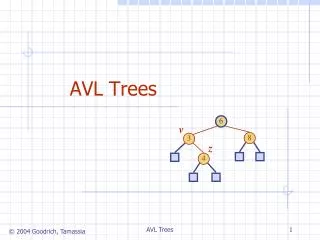
6. v. 8. 3. z. 4. AVL Trees. AVL Tree Definition (§ 9.2). AVL trees are balanced. An AVL Tree is a binary search tree such that for every internal node v of T, the heights of the children of v can differ by at most 1 .

AVL Trees
E N D
Presentation Transcript
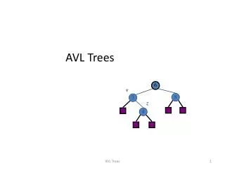
6 v 8 3 z 4 AVL Trees AVL Trees
AVL Tree Definition (§ 9.2) • AVL trees are balanced. • An AVL Tree is a binary search tree such that for every internal node v of T, the heights of the children of v can differ by at most 1. An example of an AVL tree where the heights are shown next to the nodes: AVL Trees
Balanced nodes • A internal node is balanced if the heights of its two children differ by at most 1. • Otherwise, such an internal node is unbalanced. AVL Trees
n(2) 3 n(1) 4 Height of an AVL Tree • Fact: The height of an AVL tree storing n keys is O(log n). • Proof: Let us bound n(h): the minimum number of internal nodes of an AVL tree of height h. • We easily see that n(1) = 1 and n(2) = 2 • For n > 2, an AVL tree of height h contains the root node, one AVL subtree of height n-1 and another of height n-2. • That is, n(h) = 1 + n(h-1) + n(h-2) • Knowing n(h-1) > n(h-2), we get n(h) > 2n(h-2). So n(h) > 2n(h-2), n(h) > 4n(h-4), n(h) > 8n(n-6), … (by induction), n(h) > 2in(h-2i)>2 {h/2 -1} (1) = 2 {h/2 -1} • Solving the base case we get: n(h) > 2 h/2-1 • Taking logarithms: h < 2log n(h) +2 • Thus the height of an AVL tree is O(log n) h-1 h-2 AVL Trees
44 17 78 44 32 50 88 17 78 48 62 32 50 88 54 48 62 Insertion in an AVL Tree • Insertion is as in a binary search tree • Always done by expanding an external node. • Example: c=z a=y b=x w before insertion after insertion It is no longer balanced AVL Trees
Names of important nodes • w: the newly inserted node. (insertion process follow the binary search tree method) • The heights of some nodes in T might be increased after inserting a node. • Those nodes must be on the path from w to the root. • Other nodes are not effected. • z: the first node we encounter in going up from w toward the root such that z is unbalanced. • y: the child of z with higher height. • y must be an ancestor of w. (why? Because z in unbalanced after inserting w) • x: the child of y with higher height. • The height of the sibling of x is smaller than that of x. (Otherwise, the height of y cannot be increased.) • x must be an ancestor of w. See the figure in the last slide. AVL Trees
Algorithm restructure(x): Input: A node x of a binary search tree T that has both parent y and grand-parent z. Output: Tree T after a trinode restructuring. • Let (a, b, c) be the list (increasing order) of nodes x, y, and z. Let T0, T1, T2 T3 be a left-to-right (inorder) listing of the four subtrees of x, y, and z not rooted at x, y, or z. • Replace the subtree rooted at z with a new subtree rooted at b.. • Let a be the left child of b and let T0 and T1 be the left and right subtrees of a, respectively. • Let c be the right child of b and let T2 and T3 be the left and right subtrees of c, respectively. AVL Trees
c = z b = y single rotation b = y a = x c = z a = x T T 3 0 T T T T T 0 2 1 2 3 T 1 Restructuring (as Single Rotations) • Single Rotations: AVL Trees
double rotation c = z b = x a = y a = y c = z b = x T T 3 1 T T T T T 0 0 2 3 1 T 2 Restructuring (as Double Rotations) • double rotations: AVL Trees
T T 1 1 Insertion Example, continued unbalanced... 4 44 x 3 2 17 62 z y 2 1 2 78 32 50 1 1 1 ...balanced 54 88 48 T 2 T T 0 3 AVL Trees
Theorem: • One restructure operation is enough to ensure that the whole tree is balanced. • Proof: Left to the readers. AVL Trees
Quiz 3 Misalkandiberikan data sebagaiberikut : (1,”A”), (3,”C”),(2,”B”),E,I,D,F,G,H, J • Susun data diataskedalam CBT berdasarkanindeksmenggunakan array. • Susun data diatassebagairepresentasi PQ menggunakanMinHeapTreeberdasarkanKunci • Hapus step by step dariHeapTree • Susun data diataskedalam AVL tree AVL Trees
blc = tki – tka • t = max(tki, tka) AVL Trees
Putar Kiri root pusat 1 AVL Trees
public void sisipData(int dt){ size++; // tambah jumlah node NodeAVL baru = new NodeAVL(dt); // buat node baru if (root == null) root = baru; // jika root masih null else{ // jika root tidak null NodeAVL pKini, pInduk = null; pKini = root; StackAVL st = new StackAVL(size); // buat stack // telusuri node untuk membentuk path dari root ke posisi while(pKini != null){ st.push(pKini); // simpan node pKini di stack pInduk = pKini; if (dt < pKini.data) pKini = pKini.anakKiri; else pKini = pKini.anakKanan; } AVL Trees
//sisipkan node if (!isNotSeimbang(pInduk)){ // jika sudah seimbang if(dt < pInduk.data) { pInduk.anakKiri = baru; } else { pInduk.anakKanan = baru; } ///// ----- } } else { // jika belum seimbang --> seimbangkan dulu seimbangkan(pInduk); } } } AVL Trees
//update date node induk-induknya NodeAVL pathNode; while(!st.isEmpty()) { pathNode = st.pop(); if(pathNode.anakKiri == null) pathNode.tKiri = 0; else pathNode.tKiri = pathNode.anakKiri.tinggi; if(pathNode.anakKanan == null) pathNode.tKanan = 0; else pathNode.tKanan = pathNode.anakKanan.tinggi; pathNode.seimbang = Math.abs(pathNode.tKanan - pathNode.tKiri); pathNode.tinggi = 1 + max(pathNode.tKiri, pathNode.tKanan); if (isNotSeimbang(pathNode)){ System.out.println("TESSSS"); seimbangkan(pathNode); } AVL Trees
44 17 62 32 50 78 88 48 54 Removal in an AVL Tree • Removal begins as in a binary search tree, which means the node removed will become an empty external node. Its parent, w, may cause an imbalance. • Example: 44 17 62 50 78 88 48 54 before deletion of 32 after deletion AVL Trees
Rebalancing after a Removal • Let z be the first unbalanced node encountered while travelling up the tree from w. Also, • let y be the child of z with the larger height, • let x be the child of y defined as follows; • If one of the children of y is taller than the other, choose x as the taller child of y. • If both children of y have the same height, select x be the child of y on the same side as y (i.e., if y is the left child of z, then x is the left child of y; and if y is the right child of z then x is the right child of y.) AVL Trees
Rebalancing after a Removal • We perform restructure(x) to restore balance at z. • As this restructuring may upset the balance of another node higher in the tree, we must continue checking for balance until the root of T is reached 62 44 a=z 44 78 17 62 w b=y 17 50 88 50 78 c=x 48 54 88 48 54 AVL Trees
Unbalanced after restructuring Unbalanced balanced 1 1 62 h=3 44 h=4 h=5 a=z h=5 44 78 17 62 w b=y 17 50 88 32 50 78 c=x 88 AVL Trees
Rebalancing after a Removal • We perform restructure(x) to restore balance at z. • As this restructuring may upset the balance of another node higher in the tree, we must continue checking for balance until the root of T is reached 62 44 a=z 44 78 17 62 w b=y 17 50 88 50 78 c=x 48 54 88 48 54 AVL Trees
Running Times for AVL Trees • a single restructure is O(1) • using a linked-structure binary tree • find is O(log n) • height of tree is O(log n), no restructures needed • insert is O(log n) • initial find is O(log n) • Restructuring up the tree, maintaining heights is O(log n) • remove is O(log n) • initial find is O(log n) • Restructuring up the tree, maintaining heights is O(log n) AVL Trees
7 2 9 4 2 4 7 9 7 2 2 7 9 4 4 9 7 7 2 2 9 9 4 4 Part-G1Merge Sort AVL Trees
Divide-and conquer is a general algorithm design paradigm: Divide: divide the input data S in two disjoint subsets S1and S2 Recur: solve the subproblems associated with S1and S2 Conquer: combine the solutions for S1and S2 into a solution for S The base case for the recursion are subproblems of size 0 or 1 Merge-sort is a sorting algorithm based on the divide-and-conquer paradigm Like heap-sort It uses a comparator It has O(n log n) running time Unlike heap-sort It does not use an auxiliary priority queue It accesses data in a sequential manner (suitable to sort data on a disk) Divide-and-Conquer (§ 10.1.1) AVL Trees
Merge-sort on an input sequence S with n elements consists of three steps: Divide: partition S into two sequences S1and S2 of about n/2 elements each Recur: recursively sort S1and S2 Conquer: merge S1and S2 into a unique sorted sequence Merge-Sort (§ 10.1) AlgorithmmergeSort(S, C) Inputsequence S with n elements, comparator C Outputsequence S sorted • according to C ifS.size() > 1 (S1, S2)partition(S, n/2) mergeSort(S1, C) mergeSort(S2, C) Smerge(S1, S2) AVL Trees
Merging Two Sorted Sequences Algorithmmerge(A, B) Inputsequences A and B withn/2 elements each Outputsorted sequence of A B S empty sequence whileA.isEmpty() B.isEmpty() ifA.first().element()<B.first().element() S.insertLast(A.remove(A.first())) else S.insertLast(B.remove(B.first())) whileA.isEmpty() S.insertLast(A.remove(A.first())) whileB.isEmpty() S.insertLast(B.remove(B.first())) return S • The conquer step of merge-sort consists of merging two sorted sequences A and B into a sorted sequence S containing the union of the elements of A and B • Merging two sorted sequences, each with n/2 elements and implemented by means of a doubly linked list, takes O(n) time AVL Trees
Merge-Sort Tree • An execution of merge-sort is depicted by a binary tree • each node represents a recursive call of merge-sort and stores • unsorted sequence before the execution and its partition • sorted sequence at the end of the execution • the root is the initial call • the leaves are calls on subsequences of size 0 or 1 7 2 9 4 2 4 7 9 7 2 2 7 9 4 4 9 7 7 2 2 9 9 4 4 AVL Trees
7 2 9 4 2 4 7 9 3 8 6 1 1 3 8 6 7 2 2 7 9 4 4 9 3 8 3 8 6 1 1 6 7 7 2 2 9 9 4 4 3 3 8 8 6 6 1 1 Execution Example • Partition 7 2 9 4 3 8 6 11 2 3 4 6 7 8 9 AVL Trees
7 2 2 7 9 4 4 9 3 8 3 8 6 1 1 6 7 7 2 2 9 9 4 4 3 3 8 8 6 6 1 1 Execution Example (cont.) • Recursive call, partition 7 2 9 4 3 8 6 11 2 3 4 6 7 8 9 7 2 9 4 2 4 7 9 3 8 6 1 1 3 8 6 AVL Trees
7 7 2 2 9 9 4 4 3 3 8 8 6 6 1 1 Execution Example (cont.) • Recursive call, partition 7 2 9 4 3 8 6 11 2 3 4 6 7 8 9 7 2 9 4 2 4 7 9 3 8 6 1 1 3 8 6 7 2 2 7 9 4 4 9 3 8 3 8 6 1 1 6 AVL Trees
7 2 2 7 9 4 4 9 3 8 3 8 6 1 1 6 Execution Example (cont.) • Recursive call, base case 7 2 9 4 3 8 6 11 2 3 4 6 7 8 9 7 2 9 4 2 4 7 9 3 8 6 1 1 3 8 6 77 2 2 9 9 4 4 3 3 8 8 6 6 1 1 AVL Trees
Execution Example (cont.) • Recursive call, base case 7 2 9 4 3 8 6 11 2 3 4 6 7 8 9 7 2 9 4 2 4 7 9 3 8 6 1 1 3 8 6 7 2 2 7 9 4 4 9 3 8 3 8 6 1 1 6 77 22 9 9 4 4 3 3 8 8 6 6 1 1 AVL Trees
Execution Example (cont.) • Merge 7 2 9 4 3 8 6 11 2 3 4 6 7 8 9 7 2 9 4 2 4 7 9 3 8 6 1 1 3 8 6 7 22 7 9 4 4 9 3 8 3 8 6 1 1 6 77 22 9 9 4 4 3 3 8 8 6 6 1 1 AVL Trees
Execution Example (cont.) • Recursive call, …, base case, merge 7 2 9 4 3 8 6 11 2 3 4 6 7 8 9 7 2 9 4 2 4 7 9 3 8 6 1 1 3 8 6 7 22 7 9 4 4 9 3 8 3 8 6 1 1 6 77 22 9 9 4 4 3 3 8 8 6 6 1 1 AVL Trees
Execution Example (cont.) • Merge 7 2 9 4 3 8 6 11 2 3 4 6 7 8 9 7 2 9 42 4 7 9 3 8 6 1 1 3 8 6 7 22 7 9 4 4 9 3 8 3 8 6 1 1 6 77 22 9 9 4 4 3 3 8 8 6 6 1 1 AVL Trees
Execution Example (cont.) • Recursive call, …, merge, merge 7 2 9 4 3 8 6 11 2 3 4 6 7 8 9 7 2 9 42 4 7 9 3 8 6 1 1 3 6 8 7 22 7 9 4 4 9 3 8 3 8 6 1 1 6 77 22 9 9 4 4 33 88 66 11 AVL Trees
Execution Example (cont.) • Merge 7 2 9 4 3 8 6 11 2 3 4 6 7 8 9 7 2 9 42 4 7 9 3 8 6 1 1 3 6 8 7 22 7 9 4 4 9 3 8 3 8 6 1 1 6 77 22 9 9 4 4 33 88 66 11 AVL Trees
Analysis of Merge-Sort • The height h of the merge-sort tree is O(log n) • at each recursive call we divide in half the sequence, • The overall amount or work done at the nodes of depth i is O(n) • we partition and merge 2i sequences of size n/2i • we make 2i+1 recursive calls • Thus, the total running time of merge-sort is O(n log n) AVL Trees
Summary of Sorting Algorithms AVL Trees
PR Kelompok • Susun ADT AVL Tree • Susun algoritma putar kiri, putar kanan, putar kiri kanan, putar kanan kiri, sisip data, penghapusan data. • [Implementasi ADT AVL Tree]<- menyusul • Tulis di kertas Folio bergaris • Jum’at dikumpul dan didiskusikan AVL Trees