Download
1 / 37
370 likes | 546 Views
Nonlinear properties of the FCC/TLEP final focus with respect to L *. Bogomyagkov, E. Levichev, P.Piminov Budker Institute of Nuclear Physics Novosibirsk. Outline. Introduction ( goals,assumptions , tools) FF optical blocks Comparison of nonlinear sources of FF (theoretical)

E N D
Nonlinear properties of the FCC/TLEP final focus with respect to L* Bogomyagkov, E. Levichev, P.Piminov Budker Institute of Nuclear Physics Novosibirsk
Outline • Introduction (goals,assumptions, tools) • FF optical blocks • Comparison of nonlinear sources of FF (theoretical) • Simulation results • Chromatic properties of the telescope • Conclusions Seminar at CERN, March 24th 2014
Goals, assumptions, tools • Estimate nonlinear features of TLEP final focus as a function of L* and *. Assuming domination of the vertical plane. • Design several lattices of FF (from IP to beginning of the arc) for several L*. • Close the ring with linear matrix providing tunes good for luminosity. Find DA, detuning. Optimize DA, chromatical aberrations. Seminar at CERN, March 24th 2014
Optics blocks CRAB Y2 X1 X2 Y1 First quad fringes: large strength and beta IP: Kinematic terms: extremely low IP beta -I -I Chromatic section: strong sextupoles, large beta YXCCS CRAB FFT Seminar at CERN, March 24th 2014
Final focus L*(D0) QD0 D0=0.7 m Q0: L=4.6 m, G=95 T/m @ 175 GeV D1=0.4 m Q1: L=2 m, G=96 T/m @ 175 GeV IP Seminar at CERN, March 24th 2014
Nonlinearity: figure of merit Final goal is large dynamic aperture. However, DA can’t be calculated for part of the ring. Therefore we took nonlinear detuning coefficient as FF nonlinearity figure of merit. Advantages • Perturbations are 3rd order (octupole like) and detuning is calculated by 1st order of perturbation theory: • is additive for different sources Seminar at CERN, March 24th 2014
Detuning and DA scaling Naive approach: where Octupole resonance fixed point: • zero Fourier harmonic • h resonance driving Fourier harmonic (we believe that both are of the same magnitude order) Seminar at CERN, March 24th 2014
Final quad QD0 and chromaticity Defining the QD0 focusing requirements as o = –I one can find The beta and its derivative in the end of L* are given by FF vertical chromaticity(half of FF): QD0 natural chromaticity Correction by sextupoles Note: For FF ’ corresponds to the chromatic function excitation introduced by B.Montague (LEP Note 165, 1979) Seminar at CERN, March 24th 2014
Kinematics For the extremely low * and large transverse momentum the first order correction of non-paraxiality is given by The main contribution comes from the IP and the first drift: where 2L is the distance between 2 QD0 quads around the IP and Seminar at CERN, March 24th 2014
QD0 Fringe Fields Quadrupole fringe field nonlinearity is defined by and the vertical detuning coefficient is given by Or, with above assumptions (k10 is the central strength): E.Levichev, P.Piminov, arXiv: 0903.3028 A.V.Bogomyagkov et al. IPAC13, WEPEA049, 2615 Seminar at CERN, March 24th 2014
Octupole error in QD0 An octupole field error (or corrector) in QD0: If a field quality at the quad aperture radius ra One can rewrite the vertical octupole detuning (for 2 QD0) as Seminar at CERN, March 24th 2014
Chromatic sextupoles Vertical chromatic sextupole pair separated by –I transformer gives the following coordinate transformation in the first order*) Pair of sextupoles Octupole By analogy to the octupole and using the expression for the FF chromaticity we found for the vertical detuning (2 pairs) *)A.Bogomyagkov, S.Glykhov, E.Levichev, P.Piminovhttp://arxiv.org/abs/0909.4872 Seminar at CERN, March 24th 2014
-test for different lattices Note: Different lattice versions may have different parameters. 1) CDR 2)K.Oide, FCC Kick-off Meeting, Geneva, 14 Feb 2014 3)T.M.Taylor, PAC 1985 4) H.G. Morales, TLEP Meeting, CERN, 18 Nov 2013 Seminar at CERN, March 24th 2014
Our design, different L* * = 1 mm, K1 = 0.16 m-1, Ls = 0.5 m, s= 5 cm K1(QD0)const This estimation is very approximate and just shows the trend. We did not take into account realistic beta and dispersion behavior, magnets other but QD0, etc. All these issues are included in simulation. Seminar at CERN, March 24th 2014
Theoretical conclusions • FF nonlinearities may increase as L* in high power. • Major part of the vertical nonlinearity for the extra-low beta IP comes from chromatic sextupoles due to the finite length effect. • The finite length effect in the –I sextupole pair can be improved by additional (low-strength) sextupole correctors. • Nonlinear errors in the quads with high beta may be a problem. Correction coils (for instance, the octupole one) can help. • Third order aberrations including the fringe field and kinematics can be mitigated by a set of octupole magnets located in proper beta and phase. Seminar at CERN, March 24th 2014
Simulation • Scenario: • We use the following lattice and tracking codes: MAD8 and Acceleraticum1) (BINP home made). • The FF structure is closed optically by a linear matrix . • The tunes are fixed at (0.53, 0.57) to get large luminosity . • Dynamic aperture and other nonlinear characteristics are defined from tracking. • DA is increased by additional sextupole and octupole correctors properly installed. 1)D.Einfeld, Comparison of lattice codes, 2nd NL Beam Dynamics Workshop, Diamond Light Source, 2009 Seminar at CERN, March 24th 2014
comparison for L*=0.7 m Simulation considers all quads fringes (included those strong in the Y chromatic section) and realistic beta behavior Seminar at CERN, March 24th 2014
Dynamic aperture W/o correctors With correctors Black: L* = 0.7 m Red: L* = 1 m (aperture ) Green: L* = 1.5 m (aperture ) Blue: L* = 2 m (SURPRISE! APERTURE ) x=3.24 10-5m, y=6.52 10-8m, *x=0.5m, *x=0.001m Seminar at CERN, March 24th 2014
Explanation Y chromaticity correction section is a main source of nonlinear perturbation. Produced aberration is proportional to (K2 )2 L*=0.7 m, K2=-12 m-3, y=5255 m L*=1.5 m, K2=-14 m-3 , y= 7707 m L*=2 m, K2=-14 m-3 , y= 5149 m Seminar at CERN, March 24th 2014
Conclusion • The major source of the DA limitation is the –I Y chromatic correction section through the sextupole length effect. • Simple calculation of yy confirms it well, however for details computer simulation is necessary. • DA dependence on L* is more complicated than we expected in the beginning of this study. Increase of L* will emphasize the fringes (~L*3) compare to the sextupoles (~L*2) (we saw it definitely in SuperKEKB) but for which L*? • Sextupole and octupole corrections works well. • For L*=2 m we have Ax > 100x and Ay > 700y which seems quite enough to start. Seminar at CERN, March 24th 2014
Guiding principles for FF • IR must provide small beta functions at IP. • Chromaticity of FF doublet must be compensated semi-locally. • Geometrical aberrations from the strong sextupoles pairs, FF quadrupole fringes must be cancelled in IR. • CRAB sextupole should be as close as possible to IP, at the position with low chromaticity of beta functions and phase advances to minimize its influence on dynamic aperture. • Accelerator operates at different energies therefore it is better to have no longitudinal field integral over the FF lenses. • It is better if integral of the detector longitudinal field should be compensated before each final focus lens. • FF band width should be more than ±2%. • Synchrotron radiation background should be minimized. Seminar at CERN, March 24th 2014
Telescope: optical functions Transport matrix Karl L. Brown, SLAC-PUB-4159 Convenient for matching routines Seminar at CERN, March 24th 2014
Telescope: second and third order From equations of motion Karl L. Brown, SLAC-PUB-4159 Seminar at CERN, March 24th 2014
Telescope: optical functions One vector describes chromaticities of and Seminar at CERN, March 24th 2014
Telescope: conclusions • Simplicity of the matching and understanding chromatical properties. • One vector describes chromaticities of and . Other elements of the FF region have their influence. • Sextupoles should be almost in phase with both FF quadrupoles. • It is difficult to cancel 1st order chromaticities of and simultaneously with 1st order chromaticity of phase advance. • Once tuned it does not change even if * changes. • Additional sextupoles provide knobs for higher order chromaticity tuning. Seminar at CERN, March 24th 2014
Example with L*=2m Seminar at CERN, March 24th 2014
Example with L*=2m Nonlinear aberrations optimized Nonlinear chromaticity optimized L*=2 m, K2=-14 m-3, y= 5149 m, dx=0.077 m, K2 y=72000 m-2 L*=2 m, K2=-7 m-3, y= 7711 m , dx=0.108 m, K2 y=54000 m-2 Seminar at CERN, March 24th 2014
Example with L*=2m x=0 x=-6.4e-3 y=0 y=-4.3e-5 Wx=32 Wx=3 Wy=15 Wy=4 Wx=32 Wy=15 Seminar at CERN, March 24th 2014
Example with L*=2m x=-6.4e-3 y=-4.3e-5 Additional sextupole OFF x=-6.4e-3 y=-4.3e-5 Additional sextupole ON Seminar at CERN, March 24th 2014
Example with L*=2m x=-6.4e-3 y=-4.3e-5 Additional sextupole OFF x=-6.4e-3 y=-4.3e-5 Additional sextupole ON QX0= 4 QY0= 3 QX1= -3.53 QY1= -1.63 QX2= -176 QY2= -37 QX3= -1636 QY3= -36502 QX0= 4 QY0= 3 QX1= -3.69 QY1= -1.63 QX2= -175 QY2= -37 QX3= -2048 QY3= -1826 Seminar at CERN, March 24th 2014
Why additional sextupoles work Seminar at CERN, March 24th 2014
Trajectories L*=2m Seminar at CERN, March 24th 2014
Trajectories L*=1.5m Seminar at CERN, March 24th 2014
Trajectories L*=1m Seminar at CERN, March 24th 2014
Trajectories L*=0.7m Seminar at CERN, March 24th 2014
Summary about FF quadrupoles E=175 GeV, x=2.1 nm P.Vobly for Ctau Novosibirsk E.Paoloni for SuperB Italy Seminar at CERN, March 24th 2014
Conclusions • Presented study is independent of head-on or CW collsions. • The major source of the DA limitation is the –I Y chromatic correction section through the sextupole length effect. • Sextupole and octupole corrections works well. • For L*=2 m we have Ax > 100x and Ay > 700y, band width > 2% which seems quite enough to start. • Telescopic transformations provide simplicity of the matching and understanding chromatical properties. • Sextupoles should be almost in phase with both FF quadrupoles. • Additional sextupoles provide knobs for higher order chromaticity tuning. • To define L* feedback from detector is required. • Key questions is prototype of the final focus quadrupole (CERN superconductive group ?!). • Include realistic arcs and detector field. • Energy acceptance due to beamstrahlung should be as large as possible. Seminar at CERN, March 24th 2014