Download
1 / 53
590 likes | 854 Views
Microsoft Excel 2013. Chapter 1 Creating a Worksheet and a Chart. Objectives. Describe the Excel worksheet Enter text and numbers Use the Sum button to sum a range of cells Enter a simple function Copy the contents of a cell to a range of cells using the fill handle

E N D
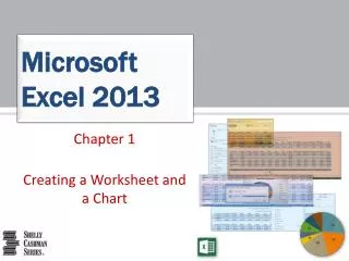
MicrosoftExcel 2013 Chapter 1 Creating a Worksheet and a Chart
Objectives • Describe the Excel worksheet • Enter text and numbers • Use the Sum button to sum a range of cells • Enter a simple function • Copy the contents of a cell to a range of cells using the fill handle • Apply cell styles • Format cells in a worksheet Creating a Worksheet and a Chart
Objectives • Create a 3-D pie chart • Change a worksheet name and worksheet tab color • Change document properties • Preview and print a worksheet • Use the AutoCalculate area to display statistics • Correct errors on a worksheet Creating a Worksheet and a Chart
Project – Worksheet and a Chart Creating a Worksheet and a Chart
Roadmap • Enter text in a blank worksheet • Calculate sums and use formulas in the worksheet • Save the workbook using a file name • Format text in the worksheet • Insert a pie chart into the worksheet • Assign a name to the worksheet tab • Preview and print the worksheet Creating a Worksheet and a Chart
Entering Worksheet Titles • Tap or click cell A1 and enter a title for the worksheet • Tap or click cell A2 andenter a subtitle • Tap or click the Enter box to complete the entry Creating a Worksheet and a Chart
Entering Column Titles • Tap or click cell A3 and enter a column title • Tap cell B3 or press the RIGHT ARROW key to enter a column title and make the cell to the right the active cell • Repeat the previous steps until all column titles are entered. Click the Enter box after entering the last column title Creating a Worksheet and a Chart
Entering Column Titles Creating a Worksheet and a Chart
Entering Row Titles • Tap or click cell A4 and enter a row title • Tap cell A5 or press the DOWN ARROW key to enter a row title and make the cell below the current cell the active cell • Repeat the previous steps until all row titles are entered Creating a Worksheet and a Chart
Entering Row Titles Creating a Worksheet and a Chart
Entering Numbers • In Excel, you can enter numbers in Excel to represent amounts • If a cell entry contains any other keyboard character, Excel interprets it as text and treats it accordingly Creating a Worksheet and a Chart
Summing a Column of Numbers • Tap or click the first empty cell below the column of numbers to sum • Tap or click the Sum button on the HOME tab to display a formula in the formula bar and in the active cell • Tap or click the Enter box in the formula bar to enter a sum in the active cell • Repeat above steps to enter the SUM function in other locations Creating a Worksheet and a Chart
Summing a Column of Numbers Creating a Worksheet and a Chart
Copying a Cell to Adjacent Cells in a Row • With the cell containing the contents to fill across the row active, tap AutoFill on the mini toolbar or point to the fill handle to activate it • Drag the fill handle to select the destination area to display a shaded border around the source area and the destination area • Lift your finger from the screen or release the mouse button to copy the SUM function from the active cell to the destination area and calculate the sums • Repeat the above steps to copy the SUM function to other ranges Creating a Worksheet and a Chart
Copying a Cell to Adjacent Cells in a Row Creating a Worksheet and a Chart
Determining Multiple Totals at the Same Time • Highlight a range at the end of rows or columns of numbers to total • Tap or click the Sum button on the HOME tab to calculate and display the sums of the corresponding rows • Repeat the above steps to calculate and display the sums of the corresponding rows Creating a Worksheet and a Chart
Determining Multiple Totals at the Same Time Creating a Worksheet and a Chart
Entering a Formula Using the Keyboard • Select the cell that will contain the formula • Type the formula in the cell to display it in the formula bar and in the current cell and to display colored borders around the cells referenced in the formula • Tap or click the cell to the right to completethe formula and to display the result in the worksheet. Creating a Worksheet and a Chart
Entering a Formula Using the Keyboard Creating a Worksheet and a Chart
Formatting the Worksheet Unformatted Worksheet Formatted Worksheet Creating a Worksheet and a Chart
Changing a Cell Style • Tap or click the desired cell and then tap or click the Cell Styles button on the HOME tab to display the Cell Styles gallery • Point to the Title cell style in the Titles and Headings area of the Cell Styles gallery to see a live preview of the cell style in the active cell • Tap or click the Title cell style to apply the cell style to the active cell Creating a Worksheet and a Chart
Changing a Cell Style Creating a Worksheet and a Chart
Changing a Font • Tap or click the desired cell for which you want to change the font • Tap or click the Font arrow on the HOME tab to display the font gallery • Point to desired font in the Font gallery to see a live preview of the selected font in the active cell • Tap or click the desired font to change the font of the selected cell Creating a Worksheet and a Chart
Changing a Font Creating a Worksheet and a Chart
Bolding a cell • Tap or click a cell to bold and then tap or click the Bold button on the HOME tab to change the font style of the active cell to bold Creating a Worksheet and a Chart
Increasing the Font Size of a Cell Entry • With the desired cell selected, tap or click the Font Size arrow on the HOME tab to display the Font Size gallery • Point to the desired font size in the Font Size gallery to see a live preview of the active cell with the selected font size • Tap or click the desired font size in the Font Size gallery to change the font size in the active cell Creating a Worksheet and a Chart
Increasing the Font Size of a Cell Entry Creating a Worksheet and a Chart
Changing the Font Color of a Cell Entry • Select the cell for which you want to change the font color and then tap or click the Font Color arrow on the HOME tab • Point to the desired color in the Theme Colors area of the Font Color gallery to see a live preview of the font color • Tap or click the desired theme to change the font color of the in the active cell Creating a Worksheet and a Chart
Changing the Font Color of a Cell Entry Creating a Worksheet and a Chart
Centering Cell Entries across Columns by Merging Cells • Drag to select the range of cells you want to merge and center • Tap or click the ‘Merge & Center’ button on the HOME tab to merge the selected range and center the contents of the leftmost cell across the selected columns • Repeat the above steps to merge and center other titles Creating a Worksheet and a Chart
Formatting Rows Using Cell Styles • Tap or click a cell and drag to select the desired range • Tap or click the Cell Styles button on the HOME tab to display the Cell Styles gallery • Tap or click a Heading cell style to apply the cell style to the selected range and then tap or click the Center button on the HOME tab to center the column headings in the selected range • Repeat the above steps to format other ranges Creating a Worksheet and a Chart
Formatting Rows Using Cell Styles Creating a Worksheet and a Chart
Formatting Numbers in the Worksheet • Select the range of cells containing numbers to format • Tap or click the desired format on the HOME tab to apply the format to the cells in the selected range Creating a Worksheet and a Chart
Adjusting the Column Width • Point to the boundary on the right side of the column of which you want to change the size to change the mouse pointer to a split double arrow • Double-click on the boundary to adjust the width of the column to the width of the largest item in the column Creating a Worksheet and a Chart
Using the Name Box to Select a Cell • Tap or click the Name box in the formula bar and then type the cell reference of the cell you wish to select • Press the ENTER key to change the active cell in the Name box Creating a Worksheet and a Chart
Other Ways to Select Cells Creating a Worksheet and a Chart
Adding a 3D Pie Chart • Select the range for the 3-D pie chart • Tap or click the ‘Insert Pie or Doughnut Chart’ button on the INSERT tabto display the Insert Pie or Doughnut Chart gallery • Tap or click the Insert Pie or Doughnut Chart gallery to insert the chart • Tap or click the chart title to select it • Type a chart title and then press the ENTER key to change the title • Deselect the chart title Creating a Worksheet and a Chart
Adding a 3D Pie Chart Creating a Worksheet and a Chart
Applying a Style to a Chart • Tap or click the Chart Styles button to display the Chart Styles gallery • Tap or click a style in the Chart Styles gallery to change the chart style to the desiredstyle Creating a Worksheet and a Chart
Moving a Chart to a New Sheet • Tap or click the Move Chart button on the CHART TOOLS DESIGN tab • Tap or click New sheet to select it and then type a title for the worksheet that will contain the chart • Tap or click the OK button to move the chart to a new chart sheet with a new sheet tab name Creating a Worksheet and a Chart
Moving a Chart to a New Sheet Creating a Worksheet and a Chart
Changing the Worksheet Tab Name • Double-tap or double-click the sheet tab you wish to change in the lower-left corner of the window • Type a new name as the worksheet tab name • Press and hold the renamed sheet tab to display a shortcut menu • Tap or point to Tab Color in the Tab Color gallery • Tap or click the desired color in the Theme Colors area to change the color of the tab Creating a Worksheet and a Chart
Changing the Worksheet Tab Name Creating a Worksheet and a Chart
Previewing and Printing a Worksheet in Landscape Orientation • In Backstage view, tap or click the Print tab to display the Print gallery • Verify that the printer listed on the Printer Status button will print a hard copy of the workbook. If necessary, click the Printer Status button to display a list of available printer options and then click the desired printer to change the currently selected printer • Tap or click the Portrait Orientation button in the Settings area and then select Landscape Orientation to change the orientation of the page to landscape. Creating a Worksheet and a Chart
Previewing and Printing a Worksheet in Landscape Orientation • Tap or click the No Scaling button and then select ‘Fit Sheet on One Page’ to print the entire worksheet on one page • Click the Print button in the Print gallery to print the worksheet in landscape orientation on the currently selected printer • When the printer stops, retrieve the hard copy Creating a Worksheet and a Chart
Previewing and Printing a Worksheet in Landscape Orientation Creating a Worksheet and a Chart
Using Common Status Bar Commands Creating a Worksheet and a Chart
Using the AutoCalculate Area to Determine a Maximum • Select the range of which you wish to determine a maximum, and then press and hold or right-click the status bar to display the Customize Status Bar shortcut menu • Tap or click Maximum on the shortcut menu to display the Maximum value in the range in the AutoCalculate area of the status bar Creating a Worksheet and a Chart
Using the AutoCalculate Area to Determine a Maximum Creating a Worksheet and a Chart
Correcting Errors after Entering Data into a Cell Creating a Worksheet and a Chart