Download

1 / 24
250 likes | 434 Views
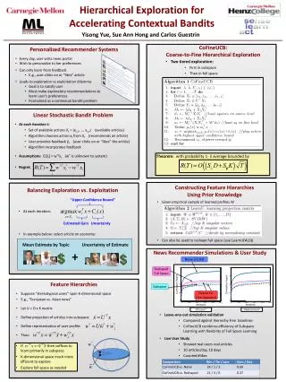
Hierarchical Exploration for Accelerating Contextual Bandits. Yisong Yue Carnegie Mellon University Joint work with Sue Ann Hong (CMU) & Carlos Guestrin (CMU). Sports. …. Like!. Politics. …. Boo!. Economy. …. Like!. Sports. …. Boo!.

E N D
Hierarchical Exploration for Accelerating Contextual Bandits Yisong Yue Carnegie Mellon University Joint work with Sue Ann Hong (CMU) & Carlos Guestrin (CMU)
Sports … Like!
Politics … Boo!
Economy … Like!
Sports … Boo!
Politics … Boo!
Politics • Exploration / Exploitation Tradeoff! • Learning “on-the-fly” • Modeled as a contextual bandit problem • Exploration is expensive • Our Goal: use prior knowledge to reduce exploration … Boo!
Linear Stochastic Bandit Problem • At time t • Set of available actions At = {at,1, …, at,n} • (articles to recommend) • Algorithm chooses action âtfrom At • (recommends an article) • User provides stochastic feedback ŷt • (user clicks on or “likes” the article) • E[ŷt] = w*Tât(w* is unknown) • Algorithm incorporates feedback • t=t+1 Regret:
Balancing Exploration vs. Exploitation “Upper Confidence Bound” • At each iteration: • Example below: select article on economy Uncertainty Estimated Gain Estimated Gain by Topic Uncertainty of Estimate +
Conventional Bandit Approach • LinUCB algorithm [Dani et al. 2008; Rusmevichientong & Tsitsiklis2008; Abbasi-Yadkori et al. 2011] • Uses particular way of defining uncertainty • Achieves regret: • Linear in dimensionality D • Linear in norm of w* How can we do better?
More Efficient Bandit Learning • LinUCB naively explores D-dimensional space • S = |w*| • Assume w* mostly in subspace • Dimensionality K << D • E.g., “European vs Asia News” • Estimated using prior knowledge • E.g., existing user profiles • Two tiered exploration • First in subspace • Then in full space • Significantly less exploration w* w* Feature Hierarchy LinUCB Guarantee:
CoFineUCB:Coarse-to-Fine Hierarchical Exploration • At time t: • Least squares in subspace • Least squares in full space • (regularized to ) • Recommend article a that maximizes • Receive feedback ŷt Uncertainty in Full Space Uncertainty in Subspace (Projection onto subspace)
Theoretical Intuition • Regret analysis of UCB algorithms requires 2 things • Rigorous confidence region of the true w* • Shrinkage rate of confidence region size • CoFineUCB uses tighter confidence regions • Can prove lies mostly in K-dim subspace • Convolution of K-dim ellipse with small D-dim ellipse
Constructing Feature Hierarchies (One Simple Approach) • Empirical sample learned user preferences • W = [w1,…,wN] • Approximately minimizes norms in regret bound • Similar to approaches for multi-task structure learning • [Argyriou et al. 2007; Zhang & Yeung 2010] • LearnU(W,K): • [A,Σ,B] = SVD(W) • (I.e., W = AΣBT) • Return U = (AΣ1/2)(1:K)/ C “Normalizing Constant”
Simulation Comparison • Leave-one-out validation using existing user profiles • From previous personalization study [Yue & Guestrin 2011] • Methods • Naïve (LinUCB) (regularize to mean of existing users) • Reshaped Full Space (LinUCB using LearnU(W,D)) • Subspace (LinUCB using LearnU(W,K)) • Often what people resort to in practice • CoFineUCB • Combines full space and subspace approaches (D=100, K = 5)
Naïve Baselines Reshaped Full space “Atypical Users” Coarse-to-Fine Approach Subspace
User Study • 10 days • 10 articles per day • From thousands of articles for that day (from Spinn3r – Jan/Feb 2012) • Submodular bandit extension to model utility of multiple articles [Yue & Guestrin 2011] • 100 topics • 5 dimensional subspace • Users rate articles • Count #likes
User Study Coarse-to-Fine Wins Coarse-to-Fine Wins ~27 users per study Ties Losses Losses LinUCB with Reshaped Full Space Naïve LinUCB *Short time horizon (T=10) made comparison with Subspace LinUCB not meaningful
Conclusions • Coarse-to-Fine approach for saving exploration • Principled approach for transferring prior knowledge • Theoretical guarantees • Depend on the quality of the constructed feature hierarchy • Validated via simulations & live user study • Future directions • Multi-level feature hierarchies • Learning feature hierarchy online • Requires learning simultaneously from multiple users • Knowledge transfer for sparse models in bandit setting Research supported by ONR (PECASE) N000141010672, ONR YIP N00014-08-1-0752, and by the Intel Science and Technology Center for Embedded Computing.
Submodular Bandit Extension • Algorithm recommends set of articles • Features depend on articles above • “Submodular basis features” • User provides stochastic feedback
CoFineLSBGreedy • At time t: • Least squares in subspace • Least squares in full space • (regularized to ) • Start with At empty • For i=1,…,L • Recommend article a that maximizes • Receive feedback yt,1,…,yt,L
Comparison with Sparse Linear Bandits • Another possible assumption: is sparse • At most B parameters are non-zero • Sparse bandit algorithms achieve regret that depend on B: • E.g., Carpentier & Munos 2011 • Limitations: • No transfer of prior knowledge • E.g., don’t know WHICH parameters are non-zero. • Typically K < B CoFineUCB achieves lower regret • E.g., fast singular value decay • S ≈ SP