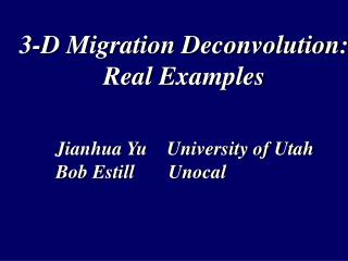
Selecting Robust Parameters for Migration Deconvolution
Selecting Robust Parameters for Migration Deconvolution. Jianhua Yu. University of Utah. Outline. Problem and Goal. Main parameter selection. Examples. Conclusions. 0.6. MD. 2-D Poststack MIG (Unocal). Depth (km). 2.8. 3-D Point Scatterer Model. 3 km. 3 km. 0. 0. Depth Slides.

Selecting Robust Parameters for Migration Deconvolution
E N D
Presentation Transcript
Selecting Robust Parameters for Migration Deconvolution Jianhua Yu University of Utah
Outline Problem and Goal Main parameter selection Examples Conclusions
0.6 MD 2-D Poststack MIG (Unocal) Depth (km) 2.8
3-D Point Scatterer Model 3 km 3 km 0 0
Depth Slides 1 km 3 km 5 km MIG MD X (km) Y (km) X (km) Y (km) 3 3 0 0 0 0 1 Amplitude
Depth Slides 7 km 9 km 10 km MIG MD X (km) Y (km) X (km) Y (km) 3 3 0 0 0 0 Amplitude
Improving the stability of MD Algorithm Developed a stable MD filter Unstable MD at some data sets Problem: Solution:
Outline Problem and Goal Main parameter selection Examples Conclusions
Blurring operator Mig: MD is to eliminate this blurring influence in migration image by designing MD operator F R = F M MD: T M = L LR T -1 Reflectivity F= (L L ) Migrated Section Prestack Migration Deconvolution
Define the MD filter length MD filter length Velocity cube Aperture width variation along the depth Calculating migration Green’s function with geometry, velocity, and depth level Inversion algorithm-regularization (Hu, 2001) Migrated cube Inverted MD fiter by inversion End of loop on iz PSMD algorithm: For iz=1, nz (depth or time slice)
N Depth Level i Depth Level 1 Depth Level N L L L N: MD filtering length L: Aperture width parameter CDP Depth (km)
For iz=1, nz (depth or time slice) Define the MD filter length Calculating migration Green’s function with the varied aperture width along the depth and associated with geometry, velocity Inverted MD filter by inversion and applied to the migrated image End of loop on iz Improved PSMD algorithm:
Outline Problem and Goal Main parameter selection Examples Conclusions
10 km 3X3 Sources; 11 X 11 Receivers 3-D Point Scatterer Model 3 km 3 km 0 0 Imaging: dx=dy=50 m dz=100 m
Z=1 km Z=3 km 0 0 0 0 0 0 0 0 0 0 0 0 X (km) X (km) X (km) X (km) X (km) X (km) Y (km) Y (km) Y (km) Y (km) Y (km) Y (km) 3 3 3 3 3 3 3 3 3 3 3 3 Z=5 km MIG MD Depth Slices
Z=7 km Z=9 km 0 0 0 0 0 0 0 0 0 0 0 0 X (km) X (km) X (km) X (km) X (km) X (km) Y (km) Y (km) Y (km) Y (km) Y (km) Y (km) 3 3 3 3 3 3 3 3 3 3 3 3 Z=10 km MIG MD Depth Slices
Z=7 km Z=9 km 0 0 0 0 0 0 0 0 0 0 0 0 X (km) X (km) X (km) X (km) X (km) X (km) Y (km) Y (km) Y (km) Y (km) Y (km) Y (km) 3 3 3 3 3 3 3 3 3 3 3 3 Z=10 km MIG MD(new) Depth Slices
Kx Kx Kx Kx Kx Kx Ky Ky Ky Ky Ky Ky Spectrum of Green’s function (Old) Spectrum of Green’s function (New) Z=1 km Z=3 km Z=5 km
Kx Kx Kx Kx Kx Kx Ky Ky Ky Ky Ky Ky Spectrum of Green’s function (Old) Spectrum of Green’s function (New) Z=7 km Z=9 km Z=10 km
Z=1 km Z=3 km 0 0 0 0 0 0 0 0 0 0 0 0 X (km) X (km) X (km) X (km) X (km) X (km) Y (km) Y (km) Y (km) Y (km) Y (km) Y (km) 3 3 3 3 3 3 3 3 3 3 3 3 Z=5 km MD MD (new) Depth Slices
Z=7 km Z=9 km 0 0 0 0 0 0 0 0 0 0 0 0 X (km) X (km) X (km) X (km) X (km) X (km) Y (km) Y (km) Y (km) Y (km) Y (km) Y (km) 3 3 3 3 3 3 3 3 3 3 3 3 Z=10 km MD MD (new) Depth Slices
Outline Problem and Goal Main parameter selection Examples: 2-D Meandering Model Conclusions
3-D Point Scatterer Model 3 km 3 km 0 0 Source: 5X5 Receiver: 21X 21
Meandering Stream Model Model PSDM Image MD
Outline Problem and Goal Main parameter selection Examples: 2-D marine data Conclusions
0.6 MD Poststack MIG from Unocal Depth (km) 2.8
0.6 MD MD Depth (km) 2.8
0.6 MD MIG Depth (km) 2.8
0.5 P-P PSTM by Unocal Time (s) MD 5
0.5 MIG Time (s) MD 5
MIG Time (s) MD
Outline Problem and Goal Main parameter selection Examples 2-D PS marine data Conclusions
X (km) 0 6 0 PS PSTM Image ( by Unocal) Time (s) 8
X (km) PSTM PSTMD 0 6 0 MD Time (s) 8
X (km) 0 6 0 PSTM PSTMD MD Time (s) 8
Outline Problem and Goal Main parameter selection Examples 2-DLand data Conclusions
Mig MD Time (s)
Outline Problem and Goal Main parameter selection Examples 3-D SEG/EAGE data Conclusions
3-D SEG/EAGE Salt Model 1.0-1.4 km
Mig (z=1 km) MD (z=1 km) X (km) X (km) 5 9.8 5 9.8 3 Y (km) 10
Outline Problem and Goal Main parameter selection Examples Conclusions
Filter length N=5-11; Parameter that controls aperture width ranges from 0.005-0.04. Aperture width and filter length in designing MD filter are two key parameters Varied aperture width in MD with the depth improved the stability of MD Conclusions
Acknowledgments • Thank Alan Leeds for his constructive suggestions and providing challenging data to test our MD in Chevron. • Thank Aramco, ChevronTaxco, and Unocal for providing the data sets • Thank 2002 UTAM sponsors for their financial support