Download
1 / 14
150 likes | 249 Views
Estimating a causal effect using observational data. Aad van der Vaart Afdeling Wiskunde, Vrije Universiteit Amsterdam Joint with Jamie Robins, Judith Lok, Richard Gill. CAUSALITY. Operational Definition : If individuals are randomly assigned to a treatment and control group,

E N D
Estimating a causal effect using observational data Aad van der Vaart Afdeling Wiskunde, Vrije Universiteit Amsterdam Joint with Jamie Robins, Judith Lok, Richard Gill
CAUSALITY Operational Definition: If individuals are randomly assigned to a treatment and control group, and the groups differ significantly after treatment, then the treatment causes the difference We want to apply this definition with observational data
Counter factuals treatment indicator A {0,1} outcome Y Given observations (A, Y) for a sample of individuals, mean treatment effect might be defined as E( Y | A=1 ) – E( Y | A=0 ) However, if treatment is not randomly assigned this is NOT what we want to know
Counter factuals (2) treatment indicator A {0,1} outcome Y outcome Y1 if individual had been treated outcome Y0 if individual had not been treated mean treatment effect E Y1 – E Y0 Unfortunately, we observe only one of Y1and Y0, namely: Y= YA
Counter factuals (3) ASSUMPTION: there exists a measured covariate Z with A (Y0, Y1 ) given Z Under ASSUMPTION: E Y1 – E Y0 = {E (Y | A=1, Z=z) - E (Y | A=1, Z=z) } dPZ(z) CONSEQUENCE: underASSUMPTION the mean treatment effect is estimable from the observed data (Y,Z,A) ASSUMPTION is more likely to hold if Z is “bigger” means “are statistically independent”
Longitudinal Data times: t0 < t1 < . . . . < tK treatments: a = (a0, a1, . . . , aK ) observed treatments: A = (A0, A1, . . . , AK ) counterfactual outcomes: Ya observed outcome: YA We are interested inE Yafor certaina
Longitudinal Data (2) times: t0 < t1 < . . . . < tK treatments: a = (a0, a1, . . . , aK ) observed treatments: A = (A0, A1, . . . , AK ) observed covariates: Z = (Z0, Z1, . . . , ZK ) ASSUMPTION: Ya Ak given ( Zk , Ak-1 ), for all k Under ASSUMPTION E Ya can be expressed in the distribution of the observed data (Y, Z, A ) “It is the task of an epidemiologist to collect enough information so that ASSUMPTION is satisfied”
Estimation and Testing • Under ASSUMPTION it is possible, in principle • to test whether treatment has effect • to estimate the mean counterfactual treatment effects A standard statistical approach would be to model and estimate all unknowns. However there are too many. We look for a “semiparametric approach” instead.
Shift function The quantile-distribution shift function is the (only monotone) function that transforms a variable “distributionally” into another variable. It is convenient to model a change in distribution.
treatment until time k outcome of this treatment shift map corresponding to these distributions, transforms into IDEA: modelby a parameter and estimate it Structural Nested Models
treatment until time k outcome of this treatment transforms into negative effect no effect tk-1 tk time Structural Nested Models (2) positive effect no effect negative effect
Under ASSUMPTION: • is distributed as • Make regression model for • Make model for g • Add as explanatory variable • Estimate g by the value such that does NOT add explanatory value. Estimation
Estimation (2) Example: if treatment A is binary, then we might use a logistic regression model We estimate (a , b, d ) by standard software for given g. The “true” g is the one such that the estimated d is zero. We can also test whether treatment has an effect at all by testing H0: d=0 in this model with Y instead of Yg .
End Lok, Gill, van der Vaart, Robins, 2004, Estimating the causal effect of a time-varying treatment on time-to-event using structural nested failure time models Lok, 2001 Statistical modelling of causal effects in time Proefschrift, Vrije Universiteit