Download
1 / 77
810 likes | 1.23k Views
VII Keynesian revolution - theory. Remark. Lectures VII and VIII – closed economy only But see Lectures XI and XII. John Maynard Keynes. 1883-1946 Cambridge, UK Thinker – economics, logic, probability

E N D
Remark • Lectures VII and VIII – closed economy only • But see Lectures XI and XII
John Maynard Keynes • 1883-1946 • Cambridge, UK • Thinker – economics, logic, probability • Practitioner – Treasury during WWI, advisor to the War Cabinet at WWII, crucial role at the birth of IMF/WB
Three postulates (1) Three basic conjectures about savings 1. Consumption function of disposable income only • - marginal propensity to consume, MPC, is positive and less than one: • Savings function • - marginal propensity to save, MPS, and
Three postulates (2) 3. Average propensity to consume • Keynes assumed that APC falls with increasing income • If this is true: danger of secular stagnation of capitalist economy (see later) Linear consumption function satisfies all three postulates After Keynes: large body of theory, huge empirical research – see Literature
VII.1.2 Marginal efficiency of investment • Ch. II : investment as a decreasing function of real interest, I=I(r), Ir<0 • Keynes called this relationship marginal efficiency of capital, later labeled as marginal efficiency of investment, MEI • Keynes assumption: MEI reflects expected return, these expectations very volatile, investment unstable and more than on interest, depends on many exogenous factors (low interest elasticity of investment) • After Keynes – more sophisticated investment functions, for our purpose here we keep simple investment function, with interest as only explanatory variable
Real vs. nominal interest • In the classical model: real interest r, in investment function only • On money markets: nominal interest i • In classical model so far we did not need nominal interest, as it was neither endogenous, neither exogenous variable of the model • In particular, in QTM, neither r, neither i has any role in demand for money • In Keynesian demand for money bellow, the decisive variable is nominal interest i • Not to complicate the explanation, a simple assumption: • Exogenous expected inflation πe and i = r + πe (Fisher equation) • More on Fisher equation and Fisher effect in later Lectures • Investment function: I = I(i- πe), Ii<0, Ii→0
Multiplier (1) • The notion of multiplier – see already previous lecture, in general form • Here we go back to the origins of the concept • Theoretical question: how does the equilibrium change, if there is - ceteris paribus – change in one of the exogenous variables (e.g. level of investment)? • Practical question during Great Depression: if there is an improvement in investors’ expectations about the future (i.e. there is an increase in autonomous investment), what is the impact on product (and employment)?
Multiplier (2) • Famous textbook explanation for a simple economy C = C(Y), Y = C + I, I exogenous and for impact of change in investment • Differentiation of equilibrium condition: • The term is (given the assumption on MPC) higher than one and reflects (approximately) impact of change in investment on the product • Alternatively: sum of expenditures’ increments after initial increase of AD
Keynes’ assumption on multiplier • Assumed unrealistically high levels, approaching to 3 • If this was true, than the impact of an exogenous change very strong (see next Lecture discussion on policy implications)
Classical labor market: demand, supply, flexible nominal wage, equilibrium Keynes: Does not dispute classical demand for labor Refuses the construction of the labor supply Workers do not adjust to real, but to nominal wage Nominal wage much less flexible: general political reasons after WWI (workers not ready to accept wage cuts) during Great Depression it was possible to hire labor even without increasing nominal wage On the labor market: possibility of an equilibrium with involuntary unemployment VII.1.4 Labor market, involuntary unemployment
Nominal wage rigidity and involuntary equilibrium W/P Y F Y1 Y2 W1/P2 W1/P1 N2 N3 N2 N1 N1 N N Fall of price → increase of real wage → if nominal wage rigid → unemployment N3 – N2 If equilibrium employment N2 → equilibrium output Y2, lower than full employment output Y1
VII.1.5 Liquidity preference and interest • Keynes abandoned QTM • Disregarding investment volatility – interest is a key variable for Keynes, but • It is not determined in interaction between investment and savings • It is given by equilibrium between supply and demand on the money market • Different role of interest – not as a reward for postponed consumption, but reward for giving up the possibility to hold liquid assets (money)
Why people demand money? Three different reason to demand money • Transaction demand (see QTM): people demand money to cover their transactions – increasing function of income • Precautionary demand (not much importance): people demand money to have enough cash - increasing function of income • Speculative demand (principle difference from Fisher’s version of QTM): people decide whether hold money (that provides zero interest) or any type of interest bearing asset (for simplicity called bond) • Here, in speculative money demand, nominal interest i (see remark above) Note: there is an inverse relation between interest and price of bond: the larger is interest, the lower is the price and vice versa (see any basic textbook on Finance or Macroeconomics)
Liquidity preference • Speculative demand – decreasing function of interest • Primarily, people hold liquidity (money). They give up this possibility (i.e. transfer their wealth into interest bearing bonds), only when it brings additional yield: • In general, the higher the interest, the higher the yield, hence higher interest lower demand for money (and higher demand for bonds) • Keynes: uncertainty and risk - if interest expected to increase, than price of bond very low and people prefer to hold money (why to hold bonds when their price will fall?)
Demand for money • Keynes labeled total demand for money as liquidity preference • Particular case: at very low rates of interest nobody wants to invest into bonds (everybody expects the interest to increase, so price of bond to decrease) and people hold only money (money demand is infinitely interest elastic – graphically horizontal) • Demand for money: , i M/P
Effective demand and supply determination • Aggregate demand AD: • consumption mainly given by disposable income, but has important autonomous component; relatively stable • investment, determined by expected return, very volatile, “animal spirits” • governmental expenditures exogenous • Refusal of Say’s law: • effective demand ≡ AD, supported by purchasing power (money), i.e. the demand, the agents really want to spend money for • such (effective) AD does not have to be equal to AD that would be necessary to “buy out” the full employment output • opposite causality compared to Say’s law: demand determines supply (and production, employment)
Quantitative adjustment • If consumption depends on disposable income only • If investment depends less on interest, but mainly on exogenous factors (expectations, uncertainty, etc.) • If government expenditures exogenous then • Prices are not a decisive factor in determining supply and demand on aggregate level • In equilibrating processes, producers generate output according effective AD • adjustment of quantities, not of prices • quantities, i.e. output, consumption, savings, investments, etc. adjust, not prices • Another essential novelty compared to classical model where • Output determined on labor market that adjusted to wage (price of labor) • Composition of demand determined by interest (price of money)
Equilibrium on goods market • Equilibrium condition Y=AD, so or • Solution equilibrium output • Quantitative adjustment – during the equilibrating processes, quantities, not prices, adjust • AD>AS real investment higher than planned decrease of production • AD<AS vice-versa • Graphical illustration: Paul Samuelson • Required simplification: price entirely fixed
Paul A. Samuelson • 1915 – 2009 • MIT • Neoclassical synthesis • Teacher, professor • Textbook – Economics, invented “Keynesian cross” (see next slide) • Foundation of Economic Analysis (1947) • Linear Programming and Economic Analysis • Nobel Price Award 1970
unintended investment> 0 Y,AD unintended investment< 0 E Y S,I E Y
Interest and equilibrium on the money market • Nominal supply of money exogenous, controlled by Central Bank • Supply of real money: • Equilibrium and interest determination: • Interest too high ↔ excess supply of money → people buy bonds (higher demand for bonds) → price of bond → i • Interest too low↔ excess demand for money → people sell bonds (higher supply of bonds) → price of bonds → i • Implication – by changing the supply of nominal money, Central Bank can influence the level of interest
i E
Interest and money market • Equilibrium on money market – supply of money equals demand • Principal difference from classical model: interest is determined on money market and results from • Liquidity preference • Supply of money by central authorities • Reminder: classical model – interest is a result of society’s thrift (savings) and investment demand
Consequences for labor market • If output determined on the goods market, than employment corresponds to that level of output • It does not have to be a full employment output – such an output is only a special case → main reason why Keynes called his book “General Theory” • If workers do not react to real wage → supply of labor is missing in theKeynesian model and nominal wage becomes (in particular moment of time) and exogenous variable • Equilibrium as a state of rest ↔ equilibrium with involuntary unemployment
VII.3.1 The model • Market with goods and services demand and equilibrium, assuming AD=AS supply • Labor market demand • Financial markets (money market) demand and equilibrium, assuming MD=MS • Components of aggregate demand consumption function investment function
Technical features • 6 equations and 6 endogenous variables: Y, C, I, N, P, i • Important: price P is flexible! • 5 exogenous variables: K, M, G, W, πe • Equilibrium as a state of rest • Demand equals supply on 2 markets: goods and services and money • Labor market • Nominal wage W in particular moment is given (exogenous) • Supply schedule is missing! • The model is completely interdependent, no dichotomy, money is not a veil
ISLM – important comment • Textbook interpretation (”orthodox” interpretation of Keynes): • Both prices and wages are fixed • There are spare capacities in the economy, namely the more labor can be hired without impact on the increase of wages and prices • In simple interpretation of ISLM: no need to distinguish between nominal and real interest rates (i and r), as price P is considered fixed (i.e. πe=0); bellow we use r (but coulduse i as well) • Fixed price: simplification of AD x AS relation in Keynesian model as well • Right-angled AS curve (see next slide) • Less standard derivation bellow: starting from full model,linearizing,collapsing into just two equations and getting simultaneous solution • For usual explanation of ISLM, see any textbook on macroeconomics, with graphical interpretation • Review: Appendix to this Lecture
AS P Y
John R. Hicks • 1904-1989 • LSE, Oxford • Value and Capital • Austrian school • Theories of economic growth • Nobel price (1972) • ISLM model: “Mr. Keynes and the Classics”, Econometrica, 1937
Linearization of the model Taking total differentials of all equations
IS curve Substitute (5) and (6) above into (1) to get where (7) is combination of all Y and r that satisfy equilibrium on the goods market – IS curve (investment = savings); in a (Y,r)-plane IS is decreasing (has negative slope): If in (7) we assume dY=0 and allow G vary, than i.e. with increased G, IS shifts “up and right”; and vice versa
LM curve (2) i.e. with increasing M, LM shifts to the right, and vice versa, decreasing M shifts LM to the left; respectively i.e. with increasing nominal wage W, LM shifts to the left, and vice versa, decreasing W shifts LM to the right
LM curve (1) From (3) single out dP/P and substitute into (4) to get (8) is combination of all Y and r that satisfy equilibrium on money market – LM curve (liquidity/money); in a (Y,r)-plane LM is increasing (has positive slope): If in (8) we put dY=0 and allow M to vary (keeping dW=0), respectively allow W vary (keeping dM=0), we get (see next slide):
Equilibrium as ISLM • (7) and (8) are 2 equations in 2 unknowns, Y and r • Solution: values of output and interest (and by substitution of other 4 endogenous variables) that • Ensure the equilibrium on goods and money markets • On the labor market allow for equilibrium (as state of the rest), where demand of labor does not have to be equal to labor supply r LM IS r0 Y0 Y
VII.3.3 Graphical interpretation of the full model • Full model: we distinguish between i and r again (πe≠0) • Equilibrium output determined by effective demand (ISLM) • This level of output determines the employment (on demand for labor schedule) • Demand for labor determines real wage and when nominal wage is given, then this determines price P, consistent with equilibrium on money market (with LM curve) • Equilibrium (state of rest) with involuntary unemployment
LM i NS W/P (W/P)0 i0 IS ND Y0 N0 Y N Y Y F Y0 Y0 45° Y0 Y N0 N
VII.4.1 “Keynes effect” • The model above • In the instantaneous moment of time, model allows for underemployment equilibrium – see above • Crucial assumption: exogenously given nominal wage • In reality, when we allow wage to change in time, even Keynesian model does not stay in underemployment equilibrium • Adjustment mechanism described by Keynes himself before General Theory in Treatise on Money (1930) – so-called “Keynes effect” • Excess supply of labor → W↓ → production costs ↓ → P ↓ → real money (M/P)↑ → excess supply of money, people bid bonds, i↓ and LM shifts to the right (see next slide), at the same time I↑ → AD↑ → Y↑ → N↑ • Higher AD moderates decrease of price level, so nominal wage falls faster than price (unbalanced deflation) → real wage falls • The model converges towards full employment equilibrium, underemployment equilibrium does not exists (see next slide)
LM0 i NS W/P LM1 W0/P0 i0 W1/P1 IS i1 ND Y0 Y1 N0 N1 Y N Y Y F Y1 Y1 Y0 Y0 45° Y0 Y1 Y N0 N1 N
VII.4.2 Underemployment equilibrium • Given the reality of Great Depression, Keynes was seeking for an explanation of long-lasting underemployment equilibrium • In the longer-run, nominal wage could not have been considered as fixed • When – with flexible wages - his model converges to full employment equilibrium, he needed additional assumptions to allow for a theoretical possibility of stable underemployment equilibrium • He, indeed, claims that two cases arise when underemployment equilibrium exists: • Liquidity trap • Interest-inelastic investment function
VII.4.2.1 Liquidity trap • When interest so low, that demand for money becomes infinitely interest elastic (horizontal), then • Absolute liquidity preference (nobody wants to purchase additional bonds) • Interest does not react to changes in supply of nominal money liquidity trap • LM curve becomes for some low value of interest also horizontal • Never observed in reality, in some situation, some economies close (Great Depression, Japan in the 1990s, today?)