Matrix Representation Theorems, Basis Change, and Linear Functionals in Mathematics
210 likes | 298 Views
Understanding matrix representations in linear transformations, basis changes, and linear functionals, including examples and explanations. Explore the concepts of dual spaces, annihilators, and solving linear systems.

Matrix Representation Theorems, Basis Change, and Linear Functionals in Mathematics
E N D
Presentation Transcript
Representation by matrices Representation. Basis change.
T <-> matrix of T w.r.t B and B’ • {T:V->W } <->B,B’ {Amxn } 1-1 onto • L(V,W) <->B,B’ M(m,n) 1-1 onto and is a linear isomorphism • Example: L(F2,F2) = M2x2(F) • L(Fm,Fn) = Mmxn(F) • When W=V, we often use B’=B.
Example: V = Fnx1, W=Fmx1, • T:V->W defined by T(X)=AX. • B, B’ standard basis • Then [T]B,B’ = A.
Theorem: V,W,Z, T:V->W, U:W->Zbasis B,B’,B”, A=[T]B,B’, B=[U]B’,B”. Then C = AB = [UT]B,B’’. • Matrix multiplication correspond to compositions. • Corollary: [UT]B=[U]B[T]B when V=W=Z,B=B’=B”. • Corollary. [T-1]B = ([T]B)-1 • Proof: UT=I=TU. U=T-1. [U]B[T]B=[I]B=[T]B[U]B.
Theorem 14: [T]B’=P-1[T]BP. Let U be s.t. Uaj=aj’ j=1,.., n. P=[P1,…,Pn]. Pj=[a’j]B. • Then [U]B= P and [T]B’=[U]B-1[T]B[U]B. • Examples:
Example: • B is a basis • Define
D:V->V is a differentiation. • not changed as you can compute from
Linear functionals • Linear functionals are another devices to. They are almost like vectors but are not vectors. Engineers do not distinguish them. Often one does not need to…. • They were used to be called covariant vectors. (usual vectors were called contravariant vectors) by Einstein and so on. • These distinctions help. • Dirac functionals are linear functionals. • Many singular functions are really functionals.
They are not mysterious things. • In mathematics, we give a definition and the mystery disappears (in theory). • f:V->F. V over F is a linear functional if • f(ca+b)=cf(a)+f(b), c in F, a,b in V. • If V is finite dimensional, it is easy to classify: • Define f:Fn->F by • Then f is a linear functional and is represented by a row matrix
Every linear functional is of this form: • Example: C[a,b]={f:[a,b]->R|f is continuous} is a vector space over R. • L:C[a,b] -> R, L(g)=g(x) is a linear functional. x is some point of R. • L:C[a,b]->R, L(g) = ab g(t)dt is a linear functional.
V* := L(V, F) is a vector space called the dual space. • dim V*= dim V by Theorem 5. Ch 3. • Find a basis of V*: • B={a1,…,an} is a given basis of V. • By Theorem 1 (p.69), there exists unique fi:V->F such that fi(aj)=ij for I=1,…,n, j=1,…,n. • {f1,…,fn} is a basis of V*: We only need to show they are linearly independent.
Proof: • B*={f1,…,fn} is the dual basis of V*. • Theorem 15: • (1) B* is a basis. (2) • (3) • Proof: (1) done. (2) from (*)
Proof continued: (3) • Example: l(x,y) := 2x+y defined on F2. • Basis [1,0], [0,1] • Dual basis f1(x,y):=x, f2(x,y):=y • L=2f1+f2. (f([1,0])=2, f([0,1])=1) • [x,y]=x[1,0]+y[0,1]=f1([x,y])[1,0]+f2([x,y])[0,1]
Annihilators • Definition: S a subset of V.S0 = annihilator(S) :={f:V->F|f(a)=0, for all a in V}. • S0 is a vector subspace of V*. • {0}0 = V*. V0={0}. • Theorem: W subspace of V f.d.v.s over F. dim W+ dim W0= dim V.
Proof: {a1,…,ak} basis of W. • Extend to V. {a1,…,ak,ak+1,…,an} basis of V. • {f1,…,fk,fk+1,…,fn} dual basis V*. • {fk+1,…,fn} is a basis of W0: • fk+1,…,fn are zero on a1,…,ak and hence zero on W and hence in W0. • fk+1,…,fn are independent in W0. • They span W0 : • Let f be in W0. Then
Corollary: W k-dim subspace of V. Then W is the intersection of n-k hyperspaces. • (Hyperspace: a subspace defined by one nonzero linear functional. ) • Proof: In the proof of the above theorem, W is precisely the set of vectors zero under fk+1,…,fn. Each fi gives a hyperplane. • Corollary: W1,W2 subspaces of f.d.v.s. V. Then W1=W2 iff W10=W20. • Proof: (->) obvious • (<-) If W1W2, then there exists v in W2 not in W1 (w.l.o.g). • By above corollary, there exists f in V* s.t. f(v) 0 and f|W1=0. Then f in W10 but not in W20.
Solving a linear system of equations: A11x1+…+A1nxn=0, … … …Am1x1+…+Amnxn=0. • Let fi(x1,…,xn)= Ai1x1+…+Ainxn. • The solution space is the subspace of Fn of all v s.t. fi(v)=0, i=1,…,m. • Dual point of view of this. To find the annihilators given a number of vectors: • Given vectors ai =(Ai1,…,Ain) in Fn. • Let f(x1,…,xn)= c1x1+…+cnxn .
The condition that f is in the annhilator of the subspace S span by ai is : • The solution of the system AX=0 is S0. • Thus we can apply row-reduction techniques to solve for S0. • Example 24: a1=(2,-2,3,4,-1), • a2=(-1,1,2,5,2), a3=(0,0,-1,-2,3), • a4=(1,-1,2,3,0).
![[MATRICES ]](https://cdn4.slideserve.com/144276/matrices-dt.jpg)