Enhancing Flexibility Index Analysis in Chemical Engineering Using Genetic Algorithms
470 likes | 626 Views
This seminar presentation outlines an innovative approach to flexibility index analysis in chemical engineering using genetic algorithms (GAs). The study addresses the limitations of traditional optimization methods and illustrates the application of GAs for efficiently determining the maximum parameter ranges that a design can tolerate. Topics include defining cost functions, repairing procedures for infeasible solutions, and case studies involving heat exchangers and reactor-cooler systems. The insights shared aim to advance future research in product and process design.

Enhancing Flexibility Index Analysis in Chemical Engineering Using Genetic Algorithms
E N D
Presentation Transcript
LPPD Group seminar Flexibility index analysis using geometric characteristics and Genetic Algorithm J. Moon, L. Zhang And A.A. Linninger April 5th , 2007 Laboratory for Product and Process Design, Department of Chemical Engineering, University of Illinois, Chicago, IL 60607, U.S.A.
Contents • Introduction • Flexibility analysis • Genetic algorithm • Part I – FI without control variables • Cost function definition • Repairing procedure • Case studies • Part II – FI with control variables • Characteristic of geometry with control variables • Framework for flexibility index problem with control variable • Repair procedure • Case study: • Heat Exchanger network[5][6] • Pump and pipe[3][5][6] • Reactor-cooler system • conclusion • Future work
Introduction • Flexibility index problem (analysis) • determine the maximum parameter (q) range that a design can tolerate for feasible operation • Applying traditional method for solving this problem is not efficient! • Gradient based method can find solution only with good initial guess-local solution • Maybe stochastic method (Genetic algorithm ,etc) is efficient
Introduction • Genetic algorithm • Stochastic optimization method which mimics natural selection and principles of genetics . • It is globally convergent, so good initial guess is not necessary! • One of most important aspects of GA is “to define exact cost function” which represents each chromosome’s value. • This presentation shows how Cost Function of flexibility problem is defined! START Define cost function & parameters Generate initial population Find cost for each chromosome Yes Is convergent? No Natural Selection Mating Mutation END General procedure of genetic algorithm
General concept of Repairing procedure • The ways to treat individuals not in a search space • Rejection (death Penalty): fitness =0 • Penalty : fitness- penalty: • Repairing: move illegal individuals to feasible search space • The procedure of repairing • (Local search for closet solution)-Baldwin effect • is a problem dependent (weakness) • Example • Salesman problem, knapsack problem, set covering problem • GENOCOP (GEnetic algorithm for Numerical Optimization for COnstrained Problems) Search space Repairing of infeasible individual
Nominal point Critical point Cost Function-definition • The Objective : we want to find out ‘critical point’ which : • lies on the constraints.(1st term) • Search space of GA is the boundaries of constraints • Individuals which are not on the constraints must • be killed ,get the penalty ,or be moved on one of constraints • has minimum flexibility index. (2nd term) • Cost ≈ & Penalty corresponding to distance from constraint Flexibility Index Search space + = 1st Term 2nd Term
1st Term: Repairing Procedure • 1st Term is reduced by Repairing procedure • Replacement of individuals using distance from constraint • Calculate all distances and closest points from every constraint. • Then select minimum one. • Move individual to the closest point.
1st Term: Repairing Procedure • 1st Term is reduced by Repairing process • Select dominant parameter and direction.(+-) • Move chromosome until it meets any constraint. • Dominant parameter is selected by • Direction is selected by After Repairing procedure, 1st term is diminished!
Case Study 1: non-convex two dimensional 4y+9x-198≤0 20y-(x-4)(x-8)(x-12)-240 ≤0 -y ≤0 4y+9x-198-4sin(2x)≤0 20y-(x-4)(x-8)(x-12)-240 ≤0 -y ≤0 4y+9x-198-4sin(2x)≤0 20y-(x-4)(x-8)(x-12)-240 ≤0 -y ≤0 Pop size :400,Iteration :300,Selection ratio :0.5,Mutation ratio :0.1
Case Study 2 • Convex 3D PN=(0.5,0.5,0.5) PN=(0.4,0.7,0.4)
Case Study 3 • Non-convex 3D PN=(0.8,0.5,0.8) PN=(0.8,0.5,0.8) PN=(0.5,0.5,0.5) PN=(0.5,0.5,0.5)
(-1,0) (1.5,0) (2.1,0) Actual feasible region Characteristic of geometry with control variables • Movable constraints & actual feasible region θ2 The constraints move! Z=0.0 Z=0.5 Z=1.0 θ1 z θ2 θ1 If we know the explicit expression of actual feasible region, critical point can be obtained easily! (same with problem which does not have control variables )
Characteristic of geometry with control variables • Fig 1, Flexibility index region is represented as hyper cube • Fig1, Nominal condition is represented as point • Fig 2, Flexibility index region is not represented as formal shapes • Fig 2, Nominal condition is represented as hyper cube. (not point) θ2 z F F ∆θ-=0 ∆θ-=0 θ1 θ1 Fig 1.Domain space without control variable Fig2. Domain space with control variable
θ z Θ’ projection θ1 Framework for flexibility index problem with control variable • Main optimization problem is solved by Genetic algorithm • Every individual is moved to new place using repairing procedure START Define cost function & parameters Generate initial population Θ’ Repair chromosomes z3 z2 Find cost for each chromosome z1 θ2 Yes Is convergent? θ No θN Natural Selection Mating Mutation θ1 END
Repair procedure • How to get new replacement of individuals ? • Other stochastic method (GA) • rSQP • … • Suggest new algorithm which is: • Zigzag movement • Does not need sensitivity information • Local optimization method • Multidimensional z, Unidimensional θ Move θ Select θ and direction Move z Move z Move θ (Initial step) Move θ Move θ Check moving direction of z Repeat until it is terminated Move z Individual movement using repairing algorithm Move θ
g2 g1 Zi θ g2 Zi g1 θ g2 Zi g1 θ Checking moving direction of Z • Procedure • G+=Max(gi(θ, zi+h)) and G-=Max(gi(θ, zi-h)) • When h <0 • Terminate it. G+<0 G- >0 G+<0, G- <0 Zi g1 θ G+>0, G- >0 h gets less than 0
z2 g2 znew Zi z1 g1 Moving direction :+ θ Movement of z & θ • Move control variable (z) • Find z2 moving z from z1 with direction until it meets constraint. • Change z value • znew=(z1+z2)/2 • Move uncertain parameter • Go until it meets constraint. • θ(i+1)= θ(i)+∆h • Two types of moving • From feasible region • From infeasible region g2 θ θnew θnew θ Zi g1 Moving direction :+ θ
Multiple starting points • This repairing algorithm is a local optimizer, so multiple starting points are needed! It gets a local solution
Termination condition • Local termination • No more movement of theta with changing one z • In case of h<0 (checking moving direction step) • Go to next z or the first z • Global termination • No more movement of θ with changing any z • θ meets boundary constraint
Multiple control variables (z) • When moving point meets local termination condition with zi • When i is 1 (first) , then i=i+1 • When i is not 1 • When any movement of θ is done with zi :i=1; • When not , i=i+1 • So movement is done with most sensitive z at first • order of z is important • More case studies about Multiple z must be done!
Flowchart of whole procedure of flexibility problem with control variables First step Move Define cost function & parameters Select zi, i=0 Generate initial population Check moving direction zi+ or zi- Repairing Y Y Is terminated? i=0 Find cost for each chromosome N N Is moved? Move z Natural Selection Y N Move θ Mating i=i+1 i=0 Is moved? Mutation No i>n Y: bmove=TRUE N:bmove=FALSE Is convergent? N Y Yes End End Repairing procedure
H2,2kW/K H1,FH1 583K 723K 1 2 T1 C2 388K 563K 2kW/K T2 Qc 3 393K C1 313K 3kW/K T3≤323K Case study1-Heat Exchanger network[5][6] • Uncertain parameter • Heat flow rate of stream, H1 :FH1 (kW/K) • Control variable • Cooling load :Qc (K) • Nominal Value: • FNH1=1kW/K • Expected deviation • ∆F+H1=0.8kW/K, ∆ F-H1=0kW/K • Constraints after eliminating the state variables Network of case study with uncertain flowrate FH1 [5]
Case study1-Heat Exchanger network[5][6] • One uncertain parameter FH1, and one control variable Qc • Starting point (1,15) Results of case study Feasible regions Repairing procedure for finding the critical point Feasible region of case study 1
∆P,k P2 P1 m D Cv ρ H,W η Case study2 –Pump and pipe[3][5][6] Design Variables Uncertain parameter
Case study2 –Pump and pipe[3][5][6] • Modifications of constraints • Constraint g3 is max range of m -> Remove • Modify control variable • Constraint g4,g5 is min and max range of control variable • Finally,
Case Study2 –Pump and pipe[3][6] Expected critical point m Nominal Point Cv’ P2 P2 m
Case Study2 –Pump and pipe[3][6] • GA parameters • pop size=800,iteration =100 • Mating method=simplex mating • h=range/100,dh=h/100 • Critical point found • (P2,m,C’v)=915.4706,11.2749,0.3036 • FI=0.6375 -similar to Flodaus[6] (0.618) C’v=0.3 C’v=120
Case Study2 –Pump and pipe[3][6] • Snapshots of repairing procedure Starting point boundary Starting point boundary
Case Study3 –Pump and pipe[5][6] ∆P,k P2 P1 m D Cv ρ H,W η Design Variables Uncertain parameter
Case Study3 –Pump and pipe[3][5][6] • Modification of constraint • Modify control variable • Constraint g4,g5 is min and max range of control variable • Finally, iteration :50 pop size=800 mating =simplex sub pop=4 h=100 dh=100
Case study4-Heat Exchanger network[5] • Energy Balance • Inequality constraints • By eliminating equality constraints • Deviation :+-10 H1,1.5kW/K H2,1kW/K T1(TN1=620K) T5(TN5=583K) 1 2 563K C1 388K 2kW/K T4 T3(TN3=388K) T2 T6 Qc 3 C2 T8(TN8=313K) 393K 3kW/K T7≤323K Network of case study with uncertain flowrate FH1 [5]
Case study4-Heat Exchanger network[5] • GA parameters • pop size=800 • iteration 50 • mating =simplex • h=ranges/50 dh=h/50
Case study5: Reactor-cooler system • Mass & Energy Balance • Inequality constraints A->B T1 F0 CA V T1 CA0 T0 T4 T2 F1 T1 A T1 Fw Tw1 Tw2 Reactor-cooler system[6] Control variable: T1,T2,Tw2
Case study5: Reactor-cooler system • Eliminating state variables Feasible region g1 FI=1 g2 g1 Feasible region when T1=389K,T2=350K ,Tw2=311.1K
Conclusion • It’s new approach for flexibility index problem. • Uses geometric characters of uncertain parameters and control variables spaces. • Uses stochastic algorithm with intelligent repairing algorithm. • Works regardless of convexity of feasible region. • Proper parameter values of GA are needed. (population size , maximum iteration, selection ratio, mutation ratio and step size for RP) • It is not superior than deterministic method, (and vise versa) but our research provides another option for flexibility index problem. • More research is needed. • Genetic algorithm is the best choice for this problem? (PSO, AH) • Another novel repairing method? • What is best mating method for this problem?
Future work • More case studies with multiple control variables • More research of movement from infeasible region (RP) • Another method, instead of current repairing procedure
Reference • Grossmann,I.; Floudas,C., “Active Constraint Strategy for Flexible Analysis in Chemical Processes” , Computers and Chemical Eng.,Vol.11(6),675-693,1986. • Floudas CA,Gumus ZH, Ierapetritou,M G “Global Optimization in Design under Uncertainty: Feasibility Test and Flexibility Index Problems” Ind. Eng Chem Res 40, 4267-4282,2001
θ z projection θ1 Framework for flexibility index problem with control variable • Main optimization problem is solved by Genetic algorithm • Every individual is moved to new place using repairing procedure START Define cost function & parameters Generate initial population Θ’ Θ’ Repair chromosomes z3 z2 Find cost for each chromosome z1 θ2 Yes Is convergent? θ No θN Natural Selection Mating Mutation θ1 END
Genetic algorithm with repairing procedure START Define cost function & parameters Generate initial population Repair chromosomes Find cost for each chromosome Is converged? Yes No Natural Selection Mating Mutation END