Download
1 / 30
300 likes | 412 Views
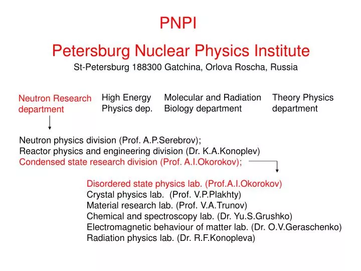
PNPI. St-Petersburg 188300 Gatchina, Orlova Roscha, Russia. Petersburg Nuclear Physics Institute. High Energy Physics dep. Molecular and Radiation Biology department. Theory Physics department. Neutron Research department. Neutron physics division (Prof. A.P.Serebrov);

E N D
PNPI St-Petersburg 188300 Gatchina, Orlova Roscha, Russia Petersburg Nuclear Physics Institute High Energy Physics dep. Molecular and Radiation Biology department Theory Physics department Neutron Research department Neutron physics division (Prof. A.P.Serebrov); Reactor physics and engineering division (Dr. K.A.Konoplev) Condensed state research division (Prof. A.I.Okorokov); Disordered state physics lab. (Prof.A.I.Okorokov) Crystal physics lab. (Prof. V.P.Plakhty) Material research lab. (Prof. V.A.Trunov) Chemical and spectroscopy lab. (Dr. Yu.S.Grushko) Electromagnetic behaviour of matter lab. (Dr. O.V.Geraschenko) Radiation physics lab. (Dr. R.F.Konopleva)
Reactor WWR-M instruments - Polarised neutrons Power 18 MWt 16 installations 6 +1 with polarized neutrons
Scheme of fields Adiabatic Nonadiabatic Adiabatic
Possibilities of 3-d analysis For scattered neutrons 1. Separation of the magnetic and nuclear scattering; 2. Separation of the elasticIel and inelastic Iin magnetic scattering; 3. Sensitivity to is <2>1/2 = 210-7 eV/1% of Pz at =10 Å and =10-3 . 4. To get information at asymptotic limits <<Г and >>Г. For the transmitted beam 1. Study of depolarisation on the domain structure 2. Study of magnetic texture 3. Distribution of magnetic field inside the sample, for example, in high TC superconductors.
Separation of I and I el in I = I = in el Because of P = ─ e(eP0) with e=q/q and q2 = k2 [Ө2 + (ω/2E)2] Elastic and inelastic components
Separation of scattering Nuclear and Multiple scattering are separated due to sum-rule: ΣP ═ ─ 1 (Elastic scattering) i (Multiple scattering part) I = x, y, z (Nuclear Scattering) (Inelastic scattering)
Elastic scattering i } - M.F.Collins et. al. With of various kinds correction on inelasticity - 3-D analysis separation without of any correction - D.Bally et al. - P.Parette, R.Kahn
Inelastic scattering Resibois - Piette dynamical scaling relation Fe _ and >>Г
Results For Fe it is obtained: • the critical exponent of correlation radius =0.67 0.01 with high accuracy; • the critical exponent of magnetic fluctuations energy • z = 2.6170.004; • the dynamical form factor F(q,) -8/5at >> (Lorentsian asymptotic is -2 ). • Isotropic magnetic heterogeneity near TC • For Pd-Fe: Magnetostriction near TC; • For ferrites: Systematic study of magnetc texture; • For superconductors: distribution of magnetic field
Principle of spin flipping Spin follows adiabatically the effective field (in the rotating frame) B(x)=B0+A'cos(πx/l) Brf(x)=A''sin(πx/l)sin(t) ω = γH ρ = 1-sin2φ/(k2+1) k = γA l/π v
Example of flipper for scattered neutrons Coils for gradient field R-F coil Shot-circuited turn Conical frame (for SANS-2 instrument of GKSS reactor) Permanent magnet for correction of gradient field for λ ≥ 3 Å
Flipper problems We have constructed and built the adiabatic resonance flipper for instrument REFSANS (Munchen), which is located in vacuum. 1. In low vacuum (10-3 atm) high R-F field (with the voltage 1000 V at the input and output of the coil) ionizes the rest of the gases. RF current starts short-circuiting to the metallic parts of the vacuum chamber. 2 Additional problem of the vacuum is cooling the system.
Completed flipper 1 Solenoid with gradient Field The box with R-F-coils inside of it Generator of R-F-current of F=81 kHz You can see the R-F coils inside of box
Flipper 1, 3 position You can see the hole between two boxes for neutron guide
Efficiency of Flipper 1 (in vacuum), > 0.22 nm .999(2) 90 cm .997 .996 .994(2) 210 cm
Flipper 2 for scattered neutrons It is conventional flipper you seen in the beginning but for λ ≥ 2 Å
Efficiency of Flipper 2 (for scattered neutrons), > 0.22 nm .997 .999(2) 275 cm .996 .998(2) 290 cm
Neutron Resonance Interferometry • Multiwave interference phenomena • Four-wave NRSE
Sketch of the fields and (k,x) diagram RES: =1/2 RES: =1/2 B Homogeneous magnetic field B0 and oscillating B1 with frequency w0 x Precession phase: j1= i(k++- k- -)dx j2 = i(k++- k+ -)dx j3= i(k++- k-+)dx j4= i(k+-- k-+)dx j5= i(k+-- k- -)dx j6= i(k-+- k- -)dx k(x) k++ k+ k+- k0 x k-+ k- k--
1 2 3= (2 + 1)/2 3’= 3= (2 + 1)/2 4’= 4= (2 - 1)/2 4= (2 - 1)/2 S.V. Grigoriev, W.H.Kraan, F.M.Mulder, M.Th.Rekveldt, Phys.Rev.A, 62 (2000) 63601
Neutron multiwave interference phenomena RES: =1/2 RES: =1/2 a B B0 l L B1 x k++ k+ b k1 One can vary = [0 - 1] One can vary B1 = [B0 ± B] k- k0 x
B SF1: =1/2 SF2: =1/2 SF3: =1/2 SF4: =1/2 SF5: =1/2 SF6: =1/2 a B0 B1 x k++ 20 21 22 23 24 25 26 N b k+ k+- x k0 N c 1 B1 6 SF1 15 20 x 15 6 1
= BRF l/(2v); = sin2() One can vary = [0 - 1] One can vary B1 = [B0 ± B] One can measure the probability R to find spin in state-(up) or state-(down) after the system of N =100 Resonant coils, so-called “QUANTUM CARPET” 2 One can vary = [0 to1] = B L/v One can vary B1 = [B0 ± B] 0 2
“QUANTUM CARPET” is governed by the simple law of Multi-Wave Interference: R = sin2(N /2)/ sin2(/2) and cos(/2) = (1- )1/2 cos(/2) = B L/v = [0 - 1] B = B1 - B0 On the picture: is varied at different N and = 1/2 The number of sub-maxima is nsub=(N-2)/2
5 DC small coils B0 B0 B1 B1 CM SF A D P DC Large coils 6 RF-coils
The EXPERIMENT has been done for the number of resonance coils N = 6 at = sin2() =1/16 and 1/2, = /12 and = /4, respectively. The value of was varied. The experiment is in good agreement with the theory. S.V. Grigoriev et.al. Phys.Rev.A, 68 (2003) 33603
Conclusion • 3-Dimensional analysis is a powerful tool • Adiabatic resonance flipper • Multiwave interference phenomena