Multiprocessors - Parallel Computing
Multiprocessors - Parallel Computing. Processor Performance. We have looked at various ways of increasing a single processor performance (Excluding VLSI techniques): Pipelining ILP Super-scalars Out-of-order execution (Scoreboarding) VLIW Cache (L1, L2, L3) Interleaved memories

Multiprocessors - Parallel Computing
E N D
Presentation Transcript
Processor Performance • We have looked at various ways of increasing a single processor performance (Excluding VLSI techniques): • Pipelining • ILP • Super-scalars • Out-of-order execution (Scoreboarding) • VLIW • Cache (L1, L2, L3) • Interleaved memories • Compilers (Loop unrolling, branch prediction, etc.) • RAID • Etc … • However, quite often even the best microprocessors are not fast enough for certain applications !!!
Example: How far will ILP go? • Infinite resources and fetch bandwidth, perfect branch prediction and renaming
When Do We Need High Performance Computing? Case1 To do a time-consuming operation in less time I am an aircraft engineer I need to run a simulation to test the stability of the wings at high speed I’d rather have the result in 5 minutes than in 5 days so that I can complete the aircraft final design sooner.
When Do We Need High Performance Computing? Case 2 To do an operation before a tighter deadline I am a weather prediction agency I am getting input from weather stations/sensors I’d like to make the forecast for tomorrow before tomorrow
When Do We Need High Performance Computing ? Case 3 To do a high number of operations per seconds I am an engineer of Amazon.com My Web server gets 10,000 hits per seconds I’d like my Web server and my databases to handle 10,000 transactions per seconds so that customers do not experience bad delays Amazon does “process” several GBytes of data per seconds
The need for High-Performance ComputersJust some examples • Automotive design: • Major automotive companies use large systems (500+ CPUs) for: • CAD-CAM, crash testing, structural integrity and aerodynamics. • Savings: approx. $1 billion per company per year. • Semiconductor industry: • Semiconductor firms use large systems (500+ CPUs) for • device electronics simulation and logic validation • Savings: approx. $1 billion per company per year. • Airlines: • System-wide logistics optimization systems on parallel systems. • Savings: approx. $100 million per airline per year.
structural biology vehicle dynamics pharmaceutical design 72-hour weather 48-hour weather chemical dynamics 3D plasma modelling 2D airfoil oil reservoir modelling Grand Challenges 1 TB 100 GB 10 GB 1 GB Storage Requirements 100 MB 10 MB 100 MFLOPS 1GFLOPS 10 GFLOPS 100 GFLOPS 1 TFLOPS Computational Performance Requirements
Weather Forecasting • Suppose the whole global atmosphere divided into cells of size 1 km 1 km 1 km to a height of 10 km (10 cells high) - about 5 108 cells. • Suppose each cell calculation requires 200 floating point operations. In one time step, 1011 floating point operations are necessary. • To forecast the weather over 7 days using 1-minute intervals, a computer operating at 1Gflops (109 floating point operations/s) – similar to the Pentium 4 - takes 106 seconds or over 10 days. • To perform calculation in 5 minutes requires a computer operating at 3.4 Tflops (3.4 1012 floating point operations/sec).
Google 2. The web server sends the query to the Index Server cluster, which matches the query to documents. 1. The user enters a query on a web form sent to the Google web server. 4. The list, with abstracts, is displayed by the web server to the user, sorted(using a secret formula involving PageRank). 3. The match is sent to the Doc Server cluster, which retrieves the documents to generate abstracts and cached copies.
Google Requirements • Google: search engine that scales at Internet growth rates • Search engines: 24x7 availability • Google : 600M queries/day, or AVERAGE of 7500 queries/s all day • Response time goal: < 0.5 s per search • Google crawls WWW and puts up new index every 2 weeks • Storage: 5.3 billion web pages, 950 million newsgroup messages, and 925 million images indexed, Millions of videos
Google • require high amounts of computation per request • A single query on Google (on average) • reads hundreds of megabytes of data • consumes tens of billions of CPU cycles • A peak request stream on Google • requires an infrastructure comparable in sizeto largest supercomputer installations • Typical google Data center: 15000 PCs (linux), 30000 disks: almost 3 petabyte! • Google application affords easy parallelization • Different queries can run on different processors • A single query can use multiple processors • because the overall index is partitioned
Multiprocessing • Multiprocessing (Parallel Processing): Concurrent execution of tasks (programs) using multiple computing, memory and interconnection resources. • Use multiple resources to solve problems faster. • Provides alternative to faster clock for performance • Assuming a doubling of effective processor performance every 2 years, 1024-Processor system can get you the performance that it would take 20 years for a single-processor system to deliver • Using multiple processors to solve a single problem • Divide problem into many small pieces • Distribute these small problems to be solved by multiple processors simultaneously
Multiprocessing • For the last 30+ years multiprocessing has been seen as the best way to produce orders of magnitude performance gains. • Double the number of processors, get double performance (less than 2 times the cost). • It turns out that the ability to develop and deliver software for multiprocessing systems has been the impediment to wide adoption.
Amdahl’s Law • A parallel program has a sequential part (e.g., I/O) and a parallel part • T1 = T1 + (1-)T1 • Tp = T1 + (1-)T1 / p • Therefore: Speedup(p) = 1 / ( + (1-)/p) = p / ( p + 1 - ) 1 / • Example: if a code is 10% sequential (i.e., = .10), the speedup will always be lower than 1 + 90/10 = 10, no matter how many processors are used!
Performance Potential Using Multiple Processors • Amdahl's Law is pessimistic (in this case) • Let s be the serial part • Let p be the part that can be parallelized n ways • Serial: SSPPPPPP • 6 processors: SSP • P • P • P • P • P • Speedup = 8/3 = 2.67 • T(n) = • As n , T(n) • Pessimistic 1 s+p/n 1 s
Amdahl’s Law Speedup 25 20 15 1000 CPUs 16 CPUs 4 CPUs 10 5 0 10% 20% 30% 40% 50% 60% 70% 80% 90% 99% % Serial
Performance Potential: Another view • Gustafson view (more widely adopted for multiprocessors) • Parallel portion increases as the problem size increases • Serial time fixed (at s) • Parallel time proportional to problem size (true most of the time) • Old Serial: SSPPPPPP • 6 processors: SSPPPPPP • PPPPPP • PPPPPP • PPPPPP • PPPPPP • PPPPPP • Hypothetical Serial: • SSPPPPPP PPPPPP PPPPPP PPPPPP PPPPPP PPPPPP • Speedup = (8+5*6)/8 = 4.75 • T'(n) = s + n*p; T'() !!!!
Amdahl vs. Gustafson-Barsis Speedup 100 80 Gustafson-Barsis 60 Amdhal 40 20 0 10% 20% 30% 40% 50% 60% 70% 80% 90% 99% % Serial
TOP 5 Most Powerful computers in the world – must be multiprocessors http://www.top500.org/
Supercomputer Style Migration (Top500) • In the last 8 years uniprocessor and SIMDs disappeared while Clusters and Constellations grew from 3% to 80% Cluster – whole computers interconnected using their I/O bus Constellation – a cluster that uses an SMP multiprocessor as the building block
Multiprocessing (usage) • Multiprocessor systems are being used for a wide variety of uses. • Redundant processing (safeguard) – fault tolerance. • Multiprocessor systems – increase throughput • Many tasks (no communication between them) • Multi-user departmental, enterprise and web servers. • Parallel computing systems – decrease execution time. • Execute large-scale applications in parallel.
Multiprocessing • Multiple resources • Computers (e.g., clusters of PCs) • CPU (e.g., shared memory computers) • ALU (e.g., multiprocessors within a single chips) • Memory • Interconnect • Tasks • Programs • Procedures • Instructions Different combinations result in different systems. Coarse-grain Fine-grain
Why did the popularity of Multiprocessors slowed down compared to the 90s • The ability to develop and deliver software for multiprocessing systems has been the impediment to wide adoption – the goal was to make programming transparent to the user (e.g., pipelining) which never happened. However, there have a lot of advances here. • The tremendous advances of microprocessors (doubling in performance every 2 years) was able to satisfy the need of 99% of the applications • It did not make a business case: vendors were only able to sell few parallel computers (< 200). As a result, they were not able to invest in designing cheap and powerful multiprocessors • Most parallel computer vendors went bankrupt by the mid-90s – there was no business.
Flynn’s Taxonomy of Computing • SISD (Single Instruction, Single Data): • Typical uniprocessor systems that we’ve studied throughout this course. • Uniprocessor systems can time share and still be SISD. • SIMD (Single Instruction, Multiple Data): • Multiple processors simultaneously executing the same instruction on different data. • Specialized applications (e.g., image processing). • MIMD (Multiple Instruction, Multiple Data): • Multiple processors autonomously executing different instructions on different data. • Keep in mind that the processors are working together to solve a single problem.
P P P P P P P P P P P P P P P P M M M M M M M M M M M M M M M M Processor Memory SIMD Systems One control unit Lockstep All Ps do the same or nothing von Neumann Computer Some Interconnection Network
M M M M C P Global Memory Interconnection Networks C P C C C C P P P P P P P P P C P M M M M MIMD Shared Memory Systems One global memory Cache Coherence All Ps have equal access to memory
M M M M C C C C Interconnection Network P P P P Cache Coherent NUMA Each P has part of the shared memory Non uniform memory access
M M M M 1110 1111 1010 1011 0110 0111 0010 0011 LAN/WAN S 1101 1010 1000 1001 0100 0101 0010 0000 0001 P P P P Interconnection Networks MIMD Distributed Memory Systems No shared memory Message Passing Topology
Programming Environment Middleware OS OS OS M M M I/O I/O I/O C C C P P P Interconnection Network Cluster Architecture Home cluster
Internet Grids Geographically distributed platforms. Dependable, consistent, pervasive, and inexpensive access to high end computing.
Many-core Era Massively Parallel Applications 100 Multi-core Era Scalar and Parallel Applications 10 Increasing HW Threads HT 1 2003 2005 2007 2009 2011 2013 Multiprocessing within a chip: Many-Core Intel predicts 100’s of cores on a chip in 2015
SIMD Parallel Computing It can be a stand-alone multiprocessor Or Embedded in a single processor for specific applications (MMX)
SIMD Applications • Applications: • Database, image processing, and signal processing. • Image processing maps very naturally onto SIMD systems. • Each processor (Execution unit) performs operations on a single pixel or neighborhood of pixels. • The operations performed are fairly straightforward and simple. • Data could be streamed into the system and operated on in real-time or close to real-time.
SIMD Operations • Image processing on SIMD systems. • Sequential pixel operations take a very long time to perform. • A 512x512 image would require 262,144 iterations through a sequential loop with each loop executing 10 instructions. That translates to 2,621,440 clock cycles (if each instruction is a single cycle) plus loop overhead. Each pixel is operated on sequentially one after another. 512x512 image
SIMD Operations • Image processing on SIMD systems. • On a SIMD system with 64x64 processors (e.g., very simple ALUs) the same operations would take 640 cycles, where each processor operates on an 8x8 set of pixels plus loop overhead. Each processor operates on an 8x8 set of pixels in parallel. Speedup due to parallelism: 2,621,440/640 = 4096 = 64x64 (number of proc.) loop overhead ignored. 512x512 image
SIMD Operations • Image processing on SIMD systems. • On a SIMD system with 512x512 processors (which is not unreasonable on SIMD machines) the same operation would take 10 cycles. Each processor operates on a single pixel in parallel. Speedup due to parallelism: 2,621,440/10 = 262,144 = 512x512 (number of proc.)! 512x512 image Notice no loop overhead!
Pentium MMX MultiMedia eXtentions • 57 new instructions • Eight 64-bit wide MMX registers • First available in 1997 • Supported on: • Intel Pentium-MMX, Pentium II, Pentium III, Pentium IV • AMD K6, K6-2, K6-3, K7 (and later) • Cyrix M2, MMX-enhanced MediaGX, Jalapeno (and later) • Gives a large speedup in many multimedia applications
MMX SIMD Operations • Example: consider an image pixel data represented as bytes. • with MMX, eight of these pixels can be packed together in a 64-bit quantity and moved into an MMX register • MMX instruction performs the arithmetic or logical operation on all eight elements in parallel • PADD(B/W/D): Addition PADDB MM1, MM2 adds 64-bit contents of MM2 to MM1, byte-by-byte any carries generated are dropped, e.g., byte A0h + 70h = 10h • PSUB(B/W/D): Subtraction
MMX: Image Dissolve Using Alpha Blending • Example: MMX instructions speed up image composition • A flower will dissolve a swan • Alpha (a standard scheme) determines the intensity of the flower • The full intensity, the flower’s 8-bit alpha value is FFh, or 255 • The equation below calculates each pixel: Result_pixel =Flower_pixel *(alpha/255) + Swan_pixel * [1-(alpha/255)] For alpha 230, the resulting pixel is 90% flower and 10% swan
SIMD Multiprocessing • It is easy to write applications for SIMD processors • The applications are limited (image processing, computer vision, etc.) • It is frequently used to speed specific applications (e.g., graphics co-processor in SGI computers) • In the late 80s and early 90s, many SIMD machines were commercially available (e.g., Connection machine has 64K ALUs, and MasPar has 16K ALUs)
Flynn’s Taxonomy of Computing • MIMD (Multiple Instruction, Multiple Data): • Multiple processors autonomously executing different instructions on different data. • Keep in mind that the processors are working together to solve a single problem. • This is a more general form of multiprocessing, and can be used in numerous applications
MIMD Architecture Instruction Stream A Instruction Stream C Instruction Stream B Unlike SIMD, MIMD computer works asynchronously. • Shared memory (tightly coupled) MIMD • Distributed memory (loosely coupled) MIMD Data Output stream A Data Input stream A Processor A Data Output stream B Processor B Data Input stream B Data Output stream C Processor C Data Input stream C
Shared Memory Multiprocessor Processor Processor Processor Processor Registers Registers Registers Registers Caches Caches Caches Caches Chipset Memory • Memory: centralized with Uniform Memory Access time(“uma”) and bus interconnect, I/O • Examples: Sun Enterprise 6000, SGI Challenge, Intel SystemPro Disk & other IO
Shared Memory Programming Model Processor Memory System Process Process load(X) store(X) X Shared variable
Shared Memory Model Virtual address spaces for a collection of processes communicating via shared addresses Machine physical address space Pn private Load Common physical addresses Store Shared portion of address space P2 private P1 private Private portion of address space P0 private
P P P P $ $ $ $ MEM Cache Coherence Problem • Processor 3 does not see the value written by processor 0 W: X = 17 R: X R: X X:17 X:42 X:42 X:42
P P P P $ $ $ $ MEM Write Through does not help • Processor 3 sees 42 in cache (does not get the correct value (17) from memory. W: X = 17 R: X R: X R: X X:17 X:17 X:42 X:42 X:42