Download
1 / 30
300 likes | 421 Views
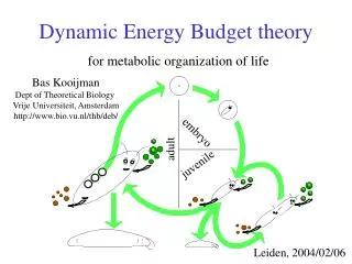
Dynamic Energy Budget theory. 1 Basic Concepts 2 Standard DEB model 3 Metabolism 4 Univariate DEB models 5 Multivariate DEB models 6 Effects of compounds 7 Extensions of DEB models 8 Co-variation of par values 9 Living together 10 Evolution 11 Evaluation.

E N D
Dynamic Energy Budget theory 1 Basic Concepts 2 Standard DEB model 3 Metabolism 4 Univariate DEB models 5 Multivariate DEB models 6 Effects of compounds 7 Extensions of DEB models 8 Co-variation of par values 9 Living together 10 Evolution 11 Evaluation
Scales of life 8a 30 Life span 10log a Volume 10log m3 earth 20 10 life on earth whale whale 0 bacterium ATP molecule -10 bacterium -20 water molecule -30
Inter-species body size scaling 8.2 • parameter values tend to co-vary across species • parameters are either intensive or extensive • ratios of extensive parameters are intensive • maximum body length is • allocation fraction to growth + maint. (intensive) • volume-specific maintenance power (intensive) • surface area-specific assimilation power (extensive) • conclusion : (so are all extensive parameters) • write physiological property as function of parameters • (including maximum body weight) • evaluate this property as function of max body weight Kooijman 1986 Energy budgets can explain body size scaling relations J. Theor. Biol.121: 269-282
Primary scaling relationships 8.2.1 assimilation {JEAm} max surface-specific assim rate Lm feeding {Fm} surface- specific searching rate digestion yEX yield of reserve on food growth yVEyield of structure on reserve mobilisation v energy conductance heating,osmosis {JET} surface-specific somatic maint. costs turnover,activity [JEM] volume-specific somatic maint. costs regulation,defence kJ maturity maintenance rate coefficient allocation partitioning fraction egg formation R reproduction efficiency life cycle MHb maturity at birth life cycle MHp maturity at puberty aging ha aging acceleration aging sG Gompertz stress coefficient Kooijman 1986 J. Theor. Biol. 121: 269-282 maximum length Lm = {JEAm} / [JEM]
Body weight 8.2.2 Body weight has contribution from structure and reserve if reproduction buffer is excluded
West-Brown: scaling of respiration 8.2.2b Explanation: Minimizing of transportation costs in space-filling fractally branching tube systems results in ¾ - “law” West et al 1997 Science276: 122-126 Problems: • Protostomes have open circulation system, no tube system scaling of respiration also applies to protostomes • Flux in capillaries is much less than in big tubes, not equal • Transport rate must match peak metabolic requirements rather than standard • No differentiation between inter- and intra-specific scaling • Transport costs are tiny fraction of maintenance costs minimum argument is not convincing (nor demonstrated) • Scaling of respiration does not explain all other scaling “laws” nor “the growth curve” of demand systems
Banavar: scaling of respiration 8.2.2c Explanation: Dilution of biomass with transport material between maintenance-requiring nodes in efficient networks results in ¾ -”law”; Banavar et al 1999 Nature399: 130-132 Problems: • Transport rate must match peak metabolic requirements rather than standard • No differentiation between inter- and intra-specific scaling • criterion • Assumption about the scaling of mass involved in transport is not tested; tubing material does not dominate in whales • Efficiency criterion is anthropomorphic
Scaling of respiration 8.2.2d Respiration: contributions from growth and maintenance Weight: contributions from structure and reserve Kooijman 1986 J Theor Biol 121: 269-282
Metabolic rate 8.2.2e slope = 1 Log metabolic rate, w O2 consumption, l/h 2 curves fitted: endotherms 0.0226 L2 + 0.0185 L3 0.0516 L2.44 ectotherms slope = 2/3 unicellulars Log weight, g Length, cm Intra-species Inter-species (Daphnia pulex) Data: Richman 1958; curve fitted from DEB theory Data: Hemmingson 1969; curve fitted from DEB theory
Feeding rate 8.2.2f slope = 1 Filtration rate, l/h Mytilus edulis Data: Winter 1973 poikilothermic tetrapods Data: Farlow 1976 Length, cm Inter-species: JXm V Intra-species: JXm V2/3
Scaling relationships 8.2.2g log scaled initial reserve log scaled age at birth log zoom factor, z log zoom factor, z approximate slope at large zoom factor log scaled length at birth log zoom factor, z
Length at puberty 8.2.2h Clupoid fishes Sardinella + Engraulis * Centengraulis Stolephorus Clupea • Brevoortia ° Sprattus Sardinops Sardina Data from Blaxter & Hunter 1982 Length at first reproduction Lp ultimate lengthL
Von Bertalanffy growth rate 8.2.2i 25 °C TA = 7 kK 10log von Bert growth rate, a-1 10log ultimate length, mm 10log ultimate length, mm ↑ ↑ 0
Body temperature of Maiasaurs 8.2.2j • determine v Bert growth rate & max length • convert length to weight (shape) • obtain v Bert growth rate for that weight at 25 °C (inter-spec) • calculate ratio with observed v Bert growth rate • convert ratio to body temperature (inverse Arrhenius) • result: 37 °C length, cm age, a
Incubation time 8.2.2k European birds tube noses 10log incubation time, d 10log incubation time, d slope = 0.25 lb equal ° tube noses 10log egg weight, g 10log egg weight, g Data from Harrison 1975 Incubation time Egg weight
Gestation time 8.2.2l Mammals * Insectivora + Primates Edentata Lagomorpha Rodentia Carnivora Proboscidea Hyracoidea Perissodactyla Artiodactyla slope = 0.33 10log gestation time, d 10log adult weight, g Data from Millar 1981 Kooijman 1986 J Theor Biol 121: 269-282
Costs for movement 8.2.2m Movement costs per distance V2/3 Investment in movement V included in somatic maintenance Home range V1/3 Data: Fedak & Seeherman , 1979 Data: Beamish, 1978 slope = -1/3 slope = -1/3 Walking costs: 5.39 ml O2 cm-2 km-1 Swimming costs: 0.65 ml O2 cm-2 km-1
Aging among species 8.2.2n Right whale slope 1/3, 1/5 Ricklefs & Finch 1995 • Conclusion for life span • hardly depends on max body size of ectotherms • increases with length in endotherms
Abundance 8.2.3 Data: Peters, 1983 feeding rate V food production constant Abundance V-1 Kooijman 1986 J Theor Biol 121: 269-282
1,1 compartment model 8.3.1 and Suppose while Kooijman et al 2004 Chemosphere 57: 745-753
Elimination rate & partition coeff 8.3.2 diffusivities low high 1 film 2 film log 10% saturation time log P01 log P01 Transition: film 1,1-compartment model Kooijman et al 2004 Chemosphere 57: 745-753
QSARs for tox parameters 8.3.4 Slope = -0.5 Slope = 1 Slope = -1 10log elim rate, d-1 10log kill rate, mM-1 d-1 10log NEC, mM 10log Pow 10log Pow 10log Pow Assumption: Each molecule has same effect Alkyl benzenes in Pimephales Data from Geiger et al 1990 • Hazard model for survival: • one compartment kinetics • hazard rate linear in internal concentration Kooijman et al 2004 Chemosphere 57: 745-753
QSARs for tox parameters 8.3.4a Slope = -0.5 Slope = 1 Slope = -1 10log elim rate, d-1 10log kill rate, mM-1 d-1 10log NEC, mM 10log Pow 10log Pow 10log Pow Benzenes, alifates, phenols in Pimephales Data from Mackay et al 1992, Hawker & Connell 1985 Assumption: Each molecule has same effect • Hazard model for survival: • one compartment kinetics • hazard rate linear in internal concentration Kooijman et al 2004 Chemosphere 57: 745-753
Covariation of tox parameters 8.3.4b Slope = -1 10log NEC, mM 10log killing rate, mM-1 d-1 Pimephales Data from Gerritsen 1997 Kooijman et al 2004 Chemosphere 57: 745-753
QSARs for LC50’s 8.3.4c 10log LC50.14d, M 10log Pow 10log Pow LC50.14d of chlorinated hydrocarbons for Poecilia. Data: Könemann, 1980
SimilaritiesQSAR body size scaling 8.4 1-compartment model: partition coefficient (= state) is ratio between uptake and elimination rate DEB-model: maximum length (= state) is ratio between assimilation and maintenance rate Parameters are constant for a system, but vary between systems in a way that follows from the model structure
InteractionsQSAR body size scaling 8.4a • uptake, elimination fluxes, food uptake surface area (intra-specifically) • elimination rate length-1 (exposure time should depend on size) • food uptake structural volume (inter-specifically) • dilution by growth affects toxicokinetics • max growth length2 (inter-specifically) • elimination via reproduction: max reprod mass flux length2 (inter-specifically) • chemical composition: reserve capacity length4 (inter-specifically) • in some taxa reserve are enriched in lipids • chemical transformation, excretion is coupled to metabolic rate • metabolic rate scales between length2 and length3 • juvenile period length, abundance length-3 , pop growth rate length-1 • links with risk assessment strategies
Dynamic Energy Budget theory 1 Basic Concepts 2 Standard DEB model 3 Metabolism 4 Univariate DEB models 5 Multivariate DEB models 6 Effects of compounds 7 Extensions of DEB models 8 Co-variation of par values 9 Living together 10 Evolution 11 Evaluation