Download
1 / 42
440 likes | 662 Views
Predicting Global Perovskite to Post-Perovskite Phase Boundary. Don Helmberger, Daoyuan Sun, Xiaodong Song, Steve Grand, Sidio Ni, and Mike Gurnis. D” region with velocity discontinuity. S-wave triplication suggests positive velocity discontinuity

E N D
Predicting Global Perovskite to Post-Perovskite Phase Boundary • Don Helmberger, Daoyuan Sun, Xiaodong Song, Steve Grand, Sidio Ni, and Mike Gurnis
D” region with velocity discontinuity • S-wave triplication suggests positive velocity discontinuity • Strong beneath the circum-Pacific lower mantle fast velocity belt • Relate to phase boundary (Perovskite to Post-Perovskite) (Grand, 2002)
D" beneath the Superplume region ? Beneath Superplume • Phase boundary is very close to CMB • Chemical distinct • Need a valid model for Superplume for exploring D"
Depth-dep. Thermal Expansion (cont.) If Drch decreases with depth. Drtotal can become negative (unstable and rise) below the height of neutral buoyancy (HNB) but positive (stable and sink) below the HNB.
Metastable Superplume • Sharp boundary • Very low velocity zone along the edge • Small scale convection features inside the Superplume
Seismic validation of the Metastable Superplume (Sdiff, ScS and PcP)
Vertical boundaries: The lower mantle beneath S. Atlantic Helmberger et al. [AGU Monograph, 2005]
3D effect for metastable Superplume model Sdpaths across the metastable Superplume
D" beneath the African Superplume region Blue circle: SKS pierce points at CMB Green Circle: ScS bounce points at CMB
D" beneath the African Superplume region Hybrid model CM model
Grand’s tomography model (2002) at the bottom mantle New phase boundary map Possible phase boundary discontinuity [Sidorin et al.,1999]
Global map of the D" The Metastable Superplume model satisfies the seismological observations for the African Superplume Phase boundary elevation A: 90 km under the African Metastable model B: 100 - 145 km (He et al., 2006) C: 160 - 345 km (Lay et al., 2006) • Is the Metastable model suitable for large anomaly beneath Central Pacific? • Difference between the middle (A) and the edge (B,C) (without down-welling cold material) of the Superplume • Difference between the Superplume region and the cold slab region • The Metastable Superplume model including phase transition at the bottom B C A
Summary • Huge Volume: 1000kmx1000kmx7000km; (Davaille,2000); evidence 1 for chemical plume • S:-3%; P 0~-0.5%,density +; evidence 2 for chemical plume ; • Sharp boundary (Ni et al, 2002; Ni and Helmberber 2003), evidence 3 for chemical plume • The shape of the superplume correlates with Geoid and Hotspots. • Tomography and geoid modeling requires higher density in the super plume. • For some regions in the lower mantle, horizontal gradients outweighs the vertical one. Thus some boundaries are more vertical than horizontal in the lower mantle.
Effect of γon phase boundary γ= 9 MPa/K, hph = 75 km γ= 3 MPa/K, hph = 140 km
Velocity discontinuity and Phase transition • Velocity Tomography model -> Non-adiabatic temperature perturbation • Determine the phase boundary with assuming Clapeyron slope (γ) and ambient phase transition elevation (hph) • Impose a velocity discontinuity (+1.5%) at the phase boundary • (Sidorin et al., 1999)